Page 354 - Matrix Analysis & Applied Linear Algebra

350 Chapter 5 Norms, Inner Products, and Orthogonality

Summary of Computational Effort
The approximate number of multiplications/divisions required to reduce
an n × n matrix to an upper-triangular form is as follows.
3
• Gaussian elimination (scaled partial pivoting) ≈ n /3.
3
• Gram–Schmidt procedure (classical and modified) ≈ n .
3
• Householder reduction ≈ 2n /3.
3
• Givens reduction ≈ 4n /3.

It’s not surprising that the unconditionally stable methods tend to be more
costly—there is no free lunch. No one triangularization technique can be con-
sidered optimal, and each has found a place in practical work. For example, in
solving unstructured linear systems, the probability of Gaussian elimination with
scaled partial pivoting failing is not high enough to justify the higher cost of using
the safer Householder or Givens reduction, or even complete pivoting. Although
much the same is true for the full-rank least squares problem, Householder re-
duction or modified Gram–Schmidt is frequently used as a safeguard against
sensitivities that often accompany least squares problems. For the purpose of
computing an orthonormal basis for R (A)in which A is unstructured and
dense (not many zeros), Householder reduction is preferred—the Gram–Schmidt
procedures are unstable for this purpose and Givens reduction is too costly.
Givens reduction is useful when the matrix being reduced is highly structured
or sparse (many zeros).

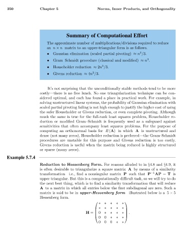
Example 5.7.4
Reduction to Hessenberg Form. For reasons alluded to in §4.8 and §4.9, it
is often desirable to triangularize a square matrix A by means of a similarity
transformation—i.e., find a nonsingular matrix P such that P −1 AP = T is
upper triangular. But this is a computationally difficult task, so we will try to do
the next best thing, which is to find a similarity transformation that will reduce
A to a matrix in which all entries below the first subdiagonal are zero. Such a
matrix is said to be in upper-Hessenberg form—illustrated below is a 5 × 5
Hessenberg form.
 
∗∗∗∗∗
 ∗∗∗∗∗ 


H =  0 ∗∗∗∗  .
 
00 ∗∗∗
000 ∗∗