Page 18 - Mechanical Engineers' Handbook (Volume 2)

2 Static Calibration 7

the ‘‘least-squares fit.’’ The principle used in making this type of curve fit is to minimize
the sum of the squares of the deviations of the data from the assumed curve. These deviations
from the assumed curve may be due to errors in one or more variables. If the error is in one
variable, the technique is called linear regression and is the common case encountered in
engineering measurements. If several variables are involved, it is called multiple regression.
Two assumptions are often used with the least-squares method: (i) the x variable (usually
the input to the calibration process) has relatively little error as compared to the y (measured)
variable and (ii) the magnitude of the uncertainty in y is not dependent on the magnitude of
the x variable. The methodology for evaluating calibration curves in systems where the
magnitude of the uncertainty in the measured value varies with the value of the input variable
can be found elsewhere. 8
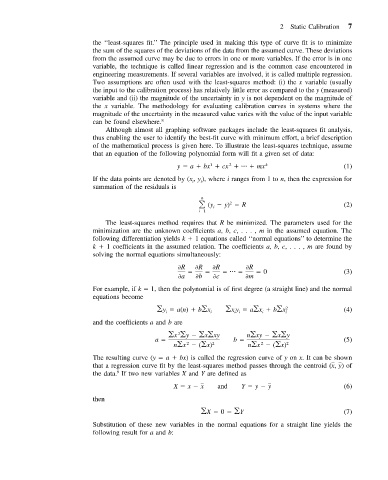
Although almost all graphing software packages include the least-squares fit analysis,
thus enabling the user to identify the best-fit curve with minimum effort, a brief description
of the mathematical process is given here. To illustrate the least-squares technique, assume
that an equation of the following polynomial form will fit a given set of data:
1
2
y a bx cx mx k (1)
If the data points are denoted by (x , y ), where i ranges from 1 to n, then the expression for
i
i
summation of the residuals is
(y y) R (2)
n
2
i 1 i
The least-squares method requires that R be minimized. The parameters used for the
minimization are the unknown coefficients a, b, c, . .., m in the assumed equation. The
following differentiation yields k 1 equations called ‘‘normal equations’’ to determine the
k 1 coefficients in the assumed relation. The coefficients a, b, c,..., m are found by
solving the normal equations simultaneously:
R R R R
0 (3)
a b c m
For example, if k 1, then the polynomial is of first degree (a straight line) and the normal
equations become
y a(n) b x xy a x b x 2 (4)
i i i i i i
and the coefficients a and b are

x y x xy n xy x y
2
a b (5)
2
2
n x ( x) 2 n x ( x) 2
The resulting curve (y a bx) is called the regression curve of y on x. It can be shown
that a regression curve fit by the least-squares method passes through the centroid (x, y ) of
the data. If two new variables X and Y are defined as
9
X x x and Y y y (6)
then
X 0 Y (7)
Substitution of these new variables in the normal equations for a straight line yields the
following result for a and b: