Page 19 - Mechanical Engineers' Handbook (Volume 2)

8 Instrument Statics

XY
a 0 b (8)
X 2
The regression line becomes
Y bX (9)
The technique described above will yield a curve based on an assumed form that will fit a
set of data. This curve may not be the best one that could be found, but it will be the best
based on the assumed form. Therefore, the ‘‘goodness of fit’’ must be determined to check
that the fitted curve follows the physical data as closely as possible.

Example 1 Choice of Functional Form. Find a suitable equation to represent the follow-
ing calibration data:
x [3, 4, 5, 7, 9, 12, 13, 14, 17, 20, 23, 25, 34, 38, 42, 45]
y [5.5, 7.75, 10.6, 13.4, 18.5, 23.6, 26.2, 27.8, 30.5, 33.5, 35, 35.4, 41, 42.1, 44.6, 46.2]

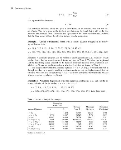
Solution: A computer program can be written or graphing software (e.g., Microsoft Excel)
used to fit the data to several assumed forms, as given in Table 1. The data can be plotted
and the best-fitting curve selected on the basis of minimum residual error, maximum cor-
relation coefficient, or smallest maximum absolute deviation, as shown in Table 1.
The analysis shows that the assumed equation y a (b) log(x) represents the best fit
through the data as it has the smallest maximum deviation and the highest correlation co-
efficient. Also note that the equation y 1/a bx is not appropriate for these data because
it has a negative correlation coefficient.

Example 2 Nonlinear Regression. Find the regression coefficients a, b, and c if the as-
2
sumed behavior of the (x, y) data is y a bx cx :
x [2, 3, 4, 5, 6, 7, 8, 9, 10, 11, 12, 13, 14, 15]
y [0.26, 0.38, 0.55, 0.70, 1.05, 1.36, 1.75, 2.20, 2.70, 3.20, 3.75, 4.40, 5.00, 6.00]

Table 1 Statistical Analysis for Example 1
Regression
Coefficient
Residual Maximum Correlation
Assumed Equation a b Error, R Deviation Coefficient a
y bx —- 1.254 56.767 10.245 0.700
y a bx 9.956 0.907 20.249 7.178 0.893
y ae bx 10.863 0.040 70.274 18.612 0.581
y 1/(a bx) 0.098 0.002 14257.327 341.451 74.302
y a b/x 40.615 133.324 32.275 9.326 0.830
y a b log x 14.188 15.612 1.542 2.791 0.992
y ax b 3.143 0.752 20.524 8.767 0.892
y x/(a bx) 0.496 0.005 48.553 14.600 0.744
a Defined in Section 4.3.7.