Page 459 - Mechanical Engineers' Handbook (Volume 2)

450 Closed-Loop Control System Analysis

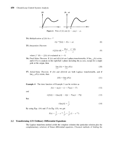
Figure 6 Plots of ƒ(t) and ƒ(t )u s (t ).

T4. Multiplication of ƒ(t) by e t
L[e t ƒ(t)] F(s ) (8)
T5. Integration Theorem
1
F(s) ƒ (0)
L[ ƒ(t) dt] (9)
s s
where ƒ (0) ƒ(t) dt evaluated at t 0.
1
T6. Final-Value Theorem. If ƒ(t) and dƒ(t)/dt are Laplace transformable, if lim t→ ƒ(t) exists,
and if F(s) is analytic in the right-half s-plane including the j axis, except for a single
pole at the origin, then
lim ƒ(t) lim sF(s) (10)
t→ s→0
T7. Initial-Value Theorem. If ƒ(t) and dƒ(t)/dt are both Laplace transformable, and if
lim s→ sF(s) exists, then

ƒ(0) lim sF(s) (11)
s→0
Example 4 The time function of Example 3 can be written as
ƒ(t) tu (t) (t T)u (t T) (12)
s
s
and
L[ƒ(t)] L[tu (t)] L[(t T)u (t T)] (13)
s
s
But
1
L[tu (t)] (14)
s
s 2
By using Eqs. (14) and (7) in Eq. (13), we get
1 1 1
F(s) e Ts (1 e Ts )
s 2 s 2 s 2

2.2 Transforming LTI Ordinary Differential Equations
The Laplace transform method yields the complete solution (the particular solution plus the
complementary solution) of linear differential equations. Classical methods of finding the