Page 823 - Mechanical Engineers' Handbook (Volume 2)

814 Neural Networks in Feedback Control Systems

Performance output Disturbance
z d
=
•
) x + (
)
)u + k
x
x = f ( f ( x + g g ( x) + k ( x ( x )d )d
u
=
y
Measured y y = x x u Control
output z =ψ= ψ ( ( , x, x ) u ) u
z
=
=
u = ( l( l( l ) y ) y ) y
u u
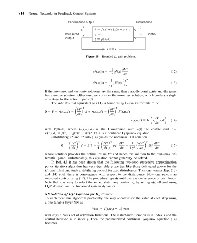
Figure 18 Bounded L 2 gain problem.
1 V*
u*(x(t)) g (x) (12)
T
2 x
1 V*
d*(x(t)) k (x) (13)
T
2 2 x
If the min–max and max–min solutions are the same, then a saddle point exists and the game
has a unique solution. Otherwise, we consider the min–max solution, which confers a slight
advantage to the action input u(t).
The infinitesimal equivalent to (11) is found using Leibniz’s formula to be
0 V r(x,u,d)
T ˙ x r(x,u,d)
T
V
V
˙
r(x,u,d) Hx, V ,u,d
x x F(x,u,d)
x (14)
with V(0) 0, where H(x,
,u,d) is the Hamiltonian with
(t) the costate and ˙x
F(x,u,d) ƒ(x) g(x)u k(x)d . This is a nonlinear Lyapunov equation.
Substituting u* and d* into (14) yields the nonlinear HJI equation
0
T ƒ hh
T T dV*
T T dV*
1 dV*
dV*
1
dV*
T
dx 4 dx gg dx 4 2 dx kk dx (15)
whose solution provides the optimal value V* and hence the solution to the min–max dif-
ferential game. Unfortunately, this equation cannot generally be solved.
In Ref. 43 it has been shown that the following two-loop successive approximation
policy iteration algorithm has very desirable properties like those delineated above for the
H case. First one finds a stabilizing control for zero disturbance. Then one iterates Eqs. (13)
2
and (14) until there is convergence with respect to the disturbance. Now one selects an
improved control using (12). The procedure repeats until there is convergence of both loops.
Note that it is easy to select the initial stabilizing control u by setting d(t) 0 and using
0
37
LQR design on the linearized system dynamics.
Control
NN Solution of HJI Equation for H
To implement this algorithm practically one may approximate the value at each step using
a one-tunable-layer NN as
T i
i
V(x) V(x,w ) w (x)
j
j
with (x) a basis set of activation functions. The disturbance iteration is in index i and the
control iteration is in index j. Then the parameterized nonlinear Lyapunov equation (14)
becomes