Page 48 - Singiresu S. Rao-Mechanical Vibrations in SI Units, Global Edition-Pearson (2017)

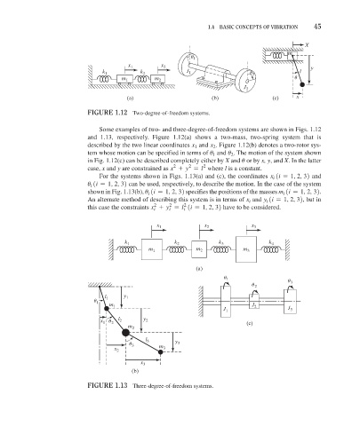
1.4 basiC ConCepts oF Vibration 45
X
m
1 u
x 1 x 2 y
k 1 k 2 J 1 2 u l
m 1 m 2 u
J 2
(a) (b) (c) x

FiGure 1.12 Two-degree-of-freedom systems.

Some examples of two- and three-degree-of-freedom systems are shown in Figs. 1.12
and 1.13, respectively. Figure 1.12(a) shows a two-mass, two-spring system that is
described by the two linear coordinates x and x . Figure 1.12(b) denotes a two-rotor sys-
2
1
tem whose motion can be specified in terms of u and u . The motion of the system shown
1
2
in Fig. 1.12(c) can be described completely either by X and u or by x, y, and X. In the latter
2
2
2
case, x and y are constrained as x + y = l where l is a constant.
For the systems shown in Figs. 1.13(a) and (c), the coordinates x 1i = 1, 2, 32 and
i
u 1i = 1, 2, 32 can be used, respectively, to describe the motion. In the case of the system
i
shown in Fig. 1.13(b), u 1i = 1, 2, 32 specifies the positions of the masses m 1i = 1, 2, 32.
i
i
An alternate method of describing this system is in terms of x and y 1i = 1, 2, 32, but in
i
i
2
2
2
this case the constraints x + y = l 1i = 1, 2, 32 have to be considered.
i
i
i
x 1 x 2 x 3
k 1 k 2 k 3 k 4
m 1 m 2 m 3
(a)
1 u 3 u
2 u
l 1 y 1
u 1
m 1 J 2
J 1 J 3
x 1 2 u l 2 y 2 (c)
m 2
l 3 y
u 3 m 3
x 2 3
x 3
(b)

FiGure 1.13 Three-degree-of-freedom systems.