Page 298 - Mechanics Analysis Composite Materials

Chapter 6. Failure criteria and strength of laminates 283

Coefficients RII. R22 and SI?can be found as earlier from Eqs. (6.10), and we need
to use an additional strength condition to determine the coupling coefficient, Rp.
A reasonable form of this condition is F(q = -e;, ~2 = -8y, 712 = 0) = 1. This
means that while for Iql < 8; and 1~21< 8y the interaction of stresses increases
material strength under compression the combination of compressive failure stresses
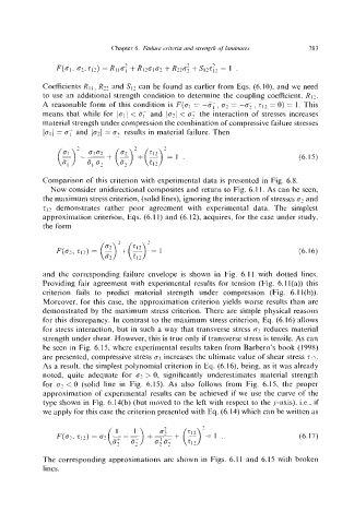
101 I = 0; and 1031 = 07 results in material failure. Then

(6.15)

Comparison of this criterion with experimental data is presented in Fig. 6.8.
Now consider unidirectional composites and return to Fig. 6.1I. As can be seen,
the maximum stress criterion, (solid lines), ignoring the interaction of stresses 02 and
212 demonstrates rather poor agreement with experimental data. The simplest
approximation criterion, Eqs. (6.1 1) and (6.12), acquires, for the case under study,
the form

(6.16)

and the corresponding failure envelope is shown in Fig. 6.1 1 with dotted lines.
Providing fair agreement with experimental results for tension (Fig. 6.1 I(a)) this
criterion fails to predict material strength under compression (Fig. 6.11(b)).
Moreover, for this case, the approximation criterion yields worse results than are
demonstrated by the maximum stress criterion. There are simple physical reasons
for this discrepancy. In contrast to the maximum stress criterion, Eq. (6.16) allows
for stress interaction, but in such a way that transverse stress 02 reduces material
strength under shear. However, this is true only if transverse stress is tensile. As can
be seen in Fig. 6.15, where experimental results taken from Barbero’s book (1998)
are presented, compressive stress is2 increases the ultimate value of shear stress TI?.
As a result, the simplest polynomial criterion in Eq. (6.16), being, as it was already
noted. quite adequate for (~2> 0, significantly underestimates material strength
for c2< 0 (solid line in Fig. 6.15). As also follows from Fig. 6.15. the proper
approximation of experimental results can be achieved if we use the curve of the
type shown in Fig. 6.14(b) (but moved to the left with respect to the y-axis). Le.. if
we apply for this case the criterion presented with Eq. (6.14) which can be written as

(6.17)

The corresponding approximations are shown in Figs. 6.1 1 and 6.15 with broken
lines.