Page 77 - Mechanics of Asphalt Microstructure and Micromechanics

70 Ch a p t e r Th r e e

for the quantification of the gradient of local volume fraction based on XCT. It consists
of five steps and is briefly described as follows.
Step 1: Obtaining XCT images and recording the thickness of slices and spacing.
Step 2: Converting gray images into binary images through determining the thresh-
olding value, which is the value at which the overall void content of the specimen is the
same as that determined through physical experimental measurements.
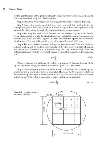
Step 3: Dividing the cross-section into squares. An inscribed square is constructed
on the binary image to study the distribution of air voids in the sample. The square was
divided into 25 small squares. Figure 3.9 shows the inscribed square and the divided
small squares. The unit in Figure 3.9 is pixel; the size of the pixel is 0.3 mm.
Step 4: The areas of voids in every small square were measured. Then, the local void
volume fraction and its gradient were calculated. By stereology principles (Equation
3-3), the volume fraction of the constituents is equal to their area fractions. Then, the
volume fraction of voids in every small square is calculated using the following equa-
tion:
a
γ = (3-11)
A
Where a denotes the total area of voids in one square, A denotes the area of the
square, and in the image, the area of every small square (A) is 449.4 mm .
2
Step 5: Calculating the gradient of the local void volume fraction. In every square,
gradients in X, Y, and Z directions are calculated. However, the formulation is different
for the small squares at the boundary and the small squares inside. For the small square
at the boundary, the following equation is used to calculate the gradient:
γ
gradφ = d (3-12a)
d

FIGURE 3.9 Inscribed square
and square division.
(76, 76) (148, 76)
1 2 3 4 5
5 72 360 (148,148) 8 9 10
7
6
(220, 220)

5 72 360