Page 113 - Mechatronic Systems Modelling and Simulation with HDLs

102 6 MECHANICS IN HARDWARE DESCRIPTION LANGUAGES

For the sake of simplicity we can also describe the cartesian coordinates of the
first body by (x 1 , x 2 , x 3 ), those of the second body by (x 4 , x 5 , x 6 ) and so on. If we
th
also term the masses of the k body m 3k−2 = m 3k−1 = m 3k and set a i = ¨x i for the
accelerations, then the equations of motion can be formulated by the following set
of equations:

e
m i ¨x i = F + F r i (i = 1, 2,... , 3N) (6.4)
i
If the movement of the particle is not restricted then the reaction forces are neg-
ligible. This yields a system of 3N second-order differential equations, which is
generally nonlinear. This equation system can in general only be solved numeri-
cally, i.e. as part of a simulation.
The constraints between the particles are characterised by a set of M independent
constraint equations:

f j (x 1 , x 2 ,..., x 3N , t) = 0 (j = 1,..., M) (6.5)

So 3N + M equations are available for the solution of the same amount of variables.
However, the use of cartesian coordinates is not always favourable. In many
cases cylindrical, spherical, elliptical, parabolic or other coordinates are benefi-
cial. For this reason we will now move to the so-called, generalised coordinates
q 1 ,...,q n . These permit a formulation that is better suited to the problem. Further-
more, under certain conditions the generalised coordinates can be selected so that
the constraint equations are dispensed with completely, considerably simplifying
the drawing up and calculation of the equations of motion. This is possible if all
constraints are holonomous, i.e. they relate exclusively to the possible geometric
positions of the bodies or can at least be put into such a form. Regardless of the
selection of coordinates, the number of degrees of freedom of the system in prin-
ciple remains constant. It corresponds with the number of independent coordinates
minus the number of independent constraint equations.
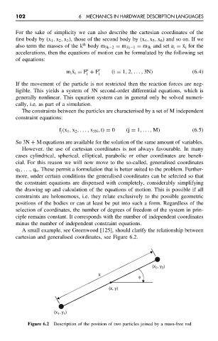
A small example, see Greenwood [125], should clarify the relationship between
cartesian and generalised coordinates, see Figure 6.2.

2
(x 2 , y )
k φ

(x, y)

(x , y )
1
1
Figure 6.2 Description of the position of two particles joined by a mass-free rod