Page 116 - Mechatronic Systems Modelling and Simulation with HDLs

6.2 MULTIBODY MECHANICS 105

 
∂x j ∂x j ∂x j
··  
˙ q 1
 ∂q 1 
∂q 2 ∂q n
   
 
v xj    ˙ q 2  v xj
 ∂y j ∂y j ∂y j   
v yj =   v yj
  ··  ·  +   (6.12)
 ∂q 1 ∂q 2 ∂q n   
v zj    ·  v zj
∂z j ∂z j ∂z j ˙ q n
 
··
∂q 1 ∂q 2 ∂q n
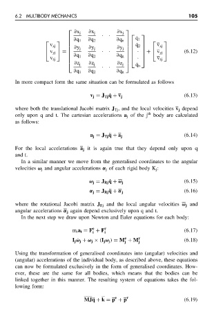
In more compact form the same situation can be formulated as follows
v j = J Tj ˙q + v j (6.13)
where both the translational Jacobi matrix J Tj , and the local velocities v j depend
only upon q and t. The cartesian accelerations a j of the j th body are calculated
as follows:

(6.14)
a j = J Tj ¨q + a j
For the local accelerations a j it is again true that they depend only upon q
and t.
In a similar manner we move from the generalised coordinates to the angular
velocities ω j and angular accelerations α j of each rigid body K j :

ω j = J Rj ˙q + ω j (6.15)
α j = J Rj ¨q + α j (6.16)

where the rotational Jacobi matrix J Rj and the local angular velocities ω j and
angular accelerations α j again depend exclusively upon q and t.
In the next step we draw upon Newton and Euler equations for each body:

e
m i a i = F + F r i (6.17)
i
e
I j ˙ω j + ω j × (I j ω j ) = M + M r j (6.18)
j
Using the transformation of generalised coordinates into (angular) velocities and
(angular) accelerations of the individual body, as described above, these equations
can now be formulated exclusively in the form of generalised coordinates. How-
ever, these are the same for all bodies, which means that the bodies can be
linked together in this manner. The resulting system of equations takes the fol-
lowing form:

e
MJ¨q + k = p + p r (6.19)