Page 351 - Microsensors, MEMS and Smart Devices - Gardner Varadhan and Awadelkarim

ACOUSTIC WAVE PROPAGATION 331

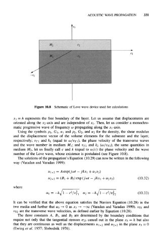
Figure 10.8 Schematic of Love wave device used for calculations

x 3 = h represents the free boundary of the layer. Let us assume that displacements are
oriented along the x 2-axis and are independent of x 1. Then, let us consider a monochro-
matic progressive wave of frequency a> propagating along the x 1-axis.
Using the symbols p 1, G 1, u 1 and P 2, G 2, and u 2 for the density, the shear modulus
and the displacement vector of the volume elements for the substrate and the layer,
respectively; VT\ and k\ (equal to CO/VTI), the phase velocity of the transverse waves
and the wave number in medium M 1; and vj2 and k 2 (<v/VT2), the same quantities in
medium A/2, let us finally call c and k (equal to cafe) the phase velocity and the wave
number of the Love wave, whose existence is postulated (see Figure 10.8).
The solutions of the propagation's Equation (10.29) can now be written in the following
way (Varadan and Varadan 1999):

jkx\
u 2x2 = (B 1 + B 2) exp (jcot - kx 1 + a 2x 3) (10.32)
j

where
2
2
2
- c /4i <*2 = -k\ - c /v T2 (10.33)
It can be verified that the above equation satisfies the Naviers Equation (10.28) in the
two media and further that u 3 ->• 0 as x 3 -> — oo (Varadan and Varadan 1999). u T1 and
are the transverse wave velocities, as defined earlier by Equation (10.28).
V T2
The three constants A, B 1, and B 2 are determined by the boundary conditions that
require not only that the tangential stresses 0 23 cancel out in the plane X 3, = h but also
that they are continuous as well as the displacements u 1x2 and u 2x2 in the plane Jt3 = 0
(Ewing et al. 1957; Slobodnik 1976).