Page 24 - Microtectonics

2.2 · Terminology 11

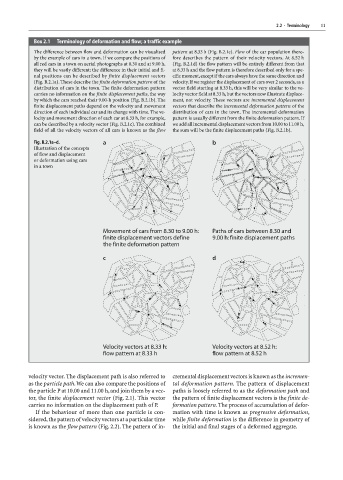
Box 2.1 Terminology of deformation and flow; a traffic example
The difference between flow and deformation can be visualised pattern at 8.33 h (Fig. B.2.1c). Flow of the car population there-
by the example of cars in a town. If we compare the positions of fore describes the pattern of their velocity vectors. At 8.52 h
all red cars in a town on aerial photographs at 8.30 and at 9.00 h, (Fig. B.2.1d) the flow pattern will be entirely different from that
they will be vastly different; the difference in their initial and fi- at 8.33 h and the flow pattern is therefore described only for a spe-
nal positions can be described by finite displacement vectors cific moment, except if the cars always have the same direction and
(Fig. B.2.1a). These describe the finite deformation pattern of the velocity. If we register the displacement of cars over 2 seconds, as a
distribution of cars in the town. The finite deformation pattern vector field starting at 8.33 h, this will be very similar to the ve-
carries no information on the finite displacement paths, the way locity vector field at 8.33 h, but the vectors now illustrate displace-
by which the cars reached their 9.00-h position (Fig. B.2.1b). The ment, not velocity. These vectors are incremental displacement
finite displacement paths depend on the velocity and movement vectors that describe the incremental deformation pattern of the
direction of each individual car and its change with time. The ve- distribution of cars in the town. The incremental deformation
locity and movement direction of each car at 8.33 h, for example, pattern is usually different from the finite deformation pattern. If
can be described by a velocity vector (Fig. B.2.1c). The combined we add all incremental displacement vectors from 10.00 to 11.00 h,
field of all the velocity vectors of all cars is known as the flow the sum will be the finite displacement paths (Fig. B.2.1b).

Fig. B.2.1a–d.
Illustration of the concepts
of flow and displacement
or deformation using cars
in a town

velocity vector. The displacement path is also referred to cremental displacement vectors is known as the incremen-
as the particle path. We can also compare the positions of tal deformation pattern. The pattern of displacement
the particle P at 10.00 and 11.00 h, and join them by a vec- paths is loosely referred to as the deformation path and
tor, the finite displacement vector (Fig. 2.1). This vector the pattern of finite displacement vectors is the finite de-
carries no information on the displacement path of P. formation pattern. The process of accumulation of defor-
If the behaviour of more than one particle is con- mation with time is known as progressive deformation,
sidered, the pattern of velocity vectors at a particular time while finite deformation is the difference in geometry of
is known as the flow pattern (Fig. 2.2). The pattern of in- the initial and final stages of a deformed aggregate.