Page 71 - Modelling in Transport Phenomena A Conceptual Approach

52 CHAPTER 3. INTERPHASE TRANSPORT

Substitution of Eq. (3.3-10) into Eq. (3.3-9) gives

(3.3-1 1)

Equation (3.3-11) indicates that the mass transfer coefficient is directly propor-
tional to the diffusion coefficient and inversely proportional to the thickness of the
concentration boundary layer.

3.3.2 Concentration at the Phase Interface
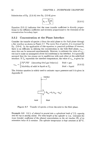
Consider the transfer of species A from the solid phase to the fluid phase through
a flat interface as shown in Figure 3.7. The molar flux of species A is expressed by
Eq. (3.3-4). In the application of this equation to practical problems of interest,
there is no difficulty in defining the concentration in the bulk fluid phase, CA,,
since this can be measured experimentally. However, to estimate the value of CA, ,
one has to make an assumption about the conditions at the interface. It is generally
assumed that the two phases are in equilibrium with each other at the solid-fluid
interface. If T, represents the interface temperature, the value of CA, is given by
A /RT (Assuming ideal gas behavior) fluid = gas
CAW = (3.3-12)
Solubility of solid in liquid at Tw fluid = liquid
The Antoine equation is widely used to estimate vapor pressures and it is given in
Appendix D.

I
Solid Fluid

Figure 3.7 Transfer of species A from the solid to the fluid phase.

Example 3.3 0.5 L of ethanol is poured into a cylindrical tank of 2 L capacity
and the top is quickly sealed The total height of the cylinder is 1 m. Calculate the
mass transfer coeficient if the ethanol concentration in the air reaches 2% of its
saturation value in 5 minutes. The cylinder temperature is kept constant at 2OOC.