Page 128 - Modern Control of DC-Based Power Systems

92 Modern Control of DC-Based Power Systems

B + ∫ C

A

–K

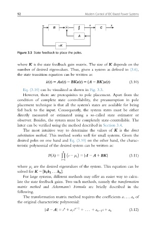
Figure 3.3 State feedback to place the poles.

where K is the state feedback gain matrix. The size of K depends on the
number of desired eigenvalues. Thus, given a system as defined in (3.6),
the state transition equation can be written as:

(3.10)
_ xtðÞ 5 Ax tðÞ 2 BKx tðÞ 5 ðA 2 BKÞxtðÞ
Eq. (3.10) can be visualized as shown in Fig. 3.3.
However, there are prerequisites to pole placement. Apart from the
condition of complete state controllability, the preassumption in pole
placement technique is that all the system’s states are available for being
fed back to the input. Consequently, the system states must be either
directly measured or estimated using a so-called state estimator or
observer. Besides, the system must be completely state-controllable. The
latter can be verified using the method described in Section 3.4.
The most intuitive way to determine the values of K is the direct
substitution method. This method works well for small systems. Given the
desired poles on one hand and Eq. (3.10) on the other hand, the charac-
teristic polynomial of the desired system can be written as:
n

(3.11)
i
j
P λ ðÞ 5 L s 2 μ 5 sI 2 A 1 BKj
i51
where μ are the desired eigenvalues of the system. This equation can be
i
solved for K 5 k 1 k 2 .. . k n Š.
½
For large systems, different methods may offer an easier way to calcu-
late the state feedback gains. Two such methods, namely the transformation
matrix method and Ackermann’s Formula are briefly described in the
following.
The transformation matrix method requires the coefficients a 1 .. . a n of
the original characteristic polynomial:

n
sI 2 Aj 5 s 1 a 1 s n21 (3.12)
j 1 .. . 1 a n21 s 1 a n