Page 385 - MODERN ELECTROCHEMISTRY

ION–ION INTERACTIONS 321

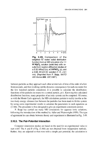
Fig. 3.49. Comparison of the
weighted -water radial distribution
function from an MD simulation of a 1.1
solution (solid line) with re-
sults from neutron diffraction studies of
a 5.32 M NaCI(o), (x), and
a 9.95 M LiCI solution (1 Å = 0.1
nm). (Reprinted from P. Bopp, NATO
ASI Series 206: 237,1987.)

between particles as they approach each other at intervals of time of the order of a few
femtoseconds, and then working out the dynamic consequences for each encounter for
the few hundred particles considered, it is possible to calculate the distribution
functions of the particles in respect to a central particle, g(r). Knowing this calculated
distribution function, many properties of an ionic system can be computed. Of course,
as with the Monte Carlo approach, the MD calculations pertain to reality insofar as the
two-body energy–distance law between the particles has been made to fit the system
by using some experimental results to calculate the parameters in such equations as
(3.166). The procedure is thus designed to give an experiment-consistent answer.
P. Bopp has carried out many MD simulations for aqueous ionic solutions,
following the introduction of the method by Adler and Wainwright (1959). The type
of agreement he can obtain between theory and experiment is illustrated in Fig. 3.49.

3.10.3. The Pair-Potential Interaction

Computer simulation studies are based on the need for an experimental value to
start with! The A and B of Eq. (3.166) are not obtained from independent methods.
Rather, they are adjusted so that even with a simple pair potential, the calculation is