Page 47 - Modern Optical Engineering The Design of Optical Systems

30 Chapter Two

and approximate calculations would have been in even better agree-
ment, yielding an image thickness of 2.502 in.

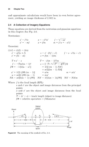
2.4 A Collection of Imagery Equations

These equations are derived from the newtonian and gaussian equations
in this chapter. See Fig. 2.6.
Newtonian:

2
x′ f /x x f /x′ f 5 22xxr
2
x′ mf x f/m m f/x x′/f
Gaussian:
(1/s′) (1/f) (1/s)
s′ sf/(s f) s s′ f/(f s′) f s s′/(s s′)
s′ f(1 m) s f(m 1)/m

2
T ≡ s′ s T f(m 1) /m
2
f Tm/(m 1) 2 s 5 [2T6 2sT 2 4fT d ]/2
f/# 1/[2(u u′)] 1/[2 (m 1) NA′]
m/[2(m 1) NA]
u′ 1/[2 (f/#) (m 1)] u/m m u/u′
u m/[2 (f/#) (m 1) mu′
NA m/[2(m 1) (f/#)] NA′ 1/[2(m 1)(f/#)] NA′ NA/m

Where f is the focal length (EFL)
s and s′ are the object and image distances from the principal
points
x and x′ are the object and image distances from the focal
points
T (s′ s) track length (object to image distance)
f/# relative aperature f/diameter

Optical
system
Object
h
m F 1 P 1 P 2 F 2 (−)µ′
(−)x (f) (f) x′
(−)h′
(−)s s′
Null T Image
space
Figure 2.6 The meaning of the symbols of Sec. 2.4.