Page 93 - Modern Optical Engineering The Design of Optical Systems

76 Chapter Five

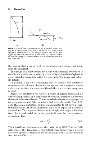
Figure 5.3 Graphical representation of spherical aberration.
(a) As a longitudinal aberration, in which the longitudinal
spherical aberration (LA′) is plotted against ray height (Y).
(b) As a transverse aberration, in which the ray intercept height
(H′) at the paraxial reference plane is plotted against the final
ray slope (tan U′).

the amount that a ray is “bent” or deviated at each surface will mini-
mize the spherical.
The image of a point formed by a lens with spherical aberration is
usually a bright dot surrounded by a halo of light; the effect of spherical
on an extended image is to soften the contrast of the image and to blur
its details.
In general, a positive, converging lens or surface will contribute
undercorrected spherical aberration to a system, and a negative lens or
a divergent surface, the reverse (although there are certain exceptions
to this).
Figure 5.3 illustrated two ways to present spherical aberration, as
either a longitudinal or a transverse aberration. Equation 5.4 showed
the relation between the two. The same relationship is also appropriate
for astigmatism and field curvature and axial chromatic (Sec. 5.3).
Note that coma, distortion, and lateral chromatic do not have a longi-
tudinal measure. All of the aberrations can also be expressed as angular
aberrations. The angular aberration is simply the angle subtended
from the second nodal (or in air, principal) point by the transverse
aberration. Thus
TA
AA (5.5)
s′
Yet a fourth way to measure an aberration is by OPD (Optical Path
Difference), the departure of the actual wave front from a perfect
reference sphere centered on the ideal image point, as discussed in
Sec. 5.6 and Chap. 15.