Page 164 - Modern Spatiotemporal Geostatistics

The Choice of a Spatiotemporal Estimate 145

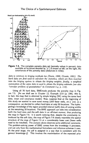
Figure 7.4. The complete porosity data set (porosity values in percent; data
available at locations denoted by "x") is shown at left; on the right, the
covariances of the porosity data (distances in miles).
data is common in kriging methods too (Davis, 1986; Cressie, 1991). The

hard data are first used to calculate the statistics, which are then inserted

into the kriging system to obtain the kriging weights; a weighted

summation of the same data is used to obtain the kriging estimate (see also
"circular problem of geostatistics" in Comment 5.4, p. 110).
Using all 76 hard data, BMEmode produces the porosity map in Fig-
ure 7.5. [As we shall see in Chapter 12, Example 12.8 (p. 239), this is,
in fact, the map that is obtained by simple kriging (SK) using the same hard
data, mean and covariance model.] Now, suppose that at the beginning of
this study we wanted to save some money (drill fewer wells, etc.) and, as a
consequence, we decided to collect hard data at only 56 locations. The hydro-
geologic knowledge of the region provided interval (soft) data of varying widths
at the remaining 20 locations. The BME approach can take into consideration
both the hard data and the soft data in an efficient manner, thus producing
the map in Figure 7.6. It is worth noticing that, despite the uncertainty in-
troduced by the soft data, the map of Figure 7.6 closely resembles the spatial
structure of the map of Figure 7.5 at a considerably lower cost (fewer wells
need to be installed). The analysis above deserves some additional comments.
The problem-solving power of BME comes from the knowledge it processes,
and not only from the mathematical formalisms and inference schemes it uses.
At the prior stage, the pdf is assigned in a way that is consistent with the
general knowledge Q. This involves the maximization of the expected prior