Page 217 - Modern Spatiotemporal Geostatistics

198 Modern Spatiotemporal Geostatistics — Chapter 10

In this chapter we will continue our study of the mathematical features
of the single-point BME model (multipoint analysis is discussed in Chapter
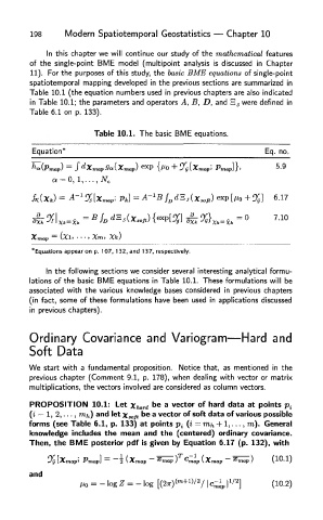
11). For the purposes of this study, the basic BME equations of single-point
spatiotemporal mapping developed in the previous sections are summarized in
Table 10.1 (the equation numbers used in previous chapters are also indicated
in Table 10.1; the parameters and operators A, B, D, and E s were defined in
Table 6.1 on p. 133).

Table 10.1. The basic BME equations.

Equation* Eq. no.

* Equations appear on p. 107, 132, and 137, respectively.
In the following sections we consider several interesting analytical formu-
lations of the basic BME equations in Table 10.1. These formulations will be
associated with the various knowledge bases considered in previous chapters
(in fact, some of these formulations have been used in applications discussed
in previous chapters).

Ordinary Covariance and Variogram—Hard and
Soft Data

We start with a fundamental proposition. Notice that, as mentioned in the
previous chapter (Comment 9.1, p. 178), when dealing with vector or matrix
multiplications, the vectors involved are considered as column vectors.

PROPOSITION 10.1: Let x hard be a vector of hard data at points p i
(i = 1, 2 , . . . , m/j) and let xaoft De a vector of soft data of various possible
forms (see Table 6.1, p. 133) at points p i (i = nth + 1,..., m). General
knowledge includes the mean and the (centered) ordinary covariance.
Then, the BME posterior pdf is given by Equation 6.17 (p. 132), with

and