Page 274 - Modern Spatiotemporal Geostatistics

Popular Methods in the Light of Modern Geostatistics 255

and time that are due to the mean of the increment; if the mean of the incre-
ment is zero, the mean of X(p) is constant). This class of models can handle
complicated space/time variabilities of any size in a mathematically rigorous
and physically meaningful manner, and is considerably more general than the
restricted class of homogeneous/stationary S/TRF (by standard convention,
the index values v = JJL = — 1 correspond to spatially homogeneous/temporally
stationary fields with no trends).
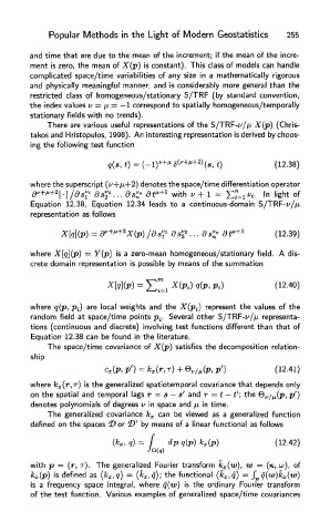
There are various useful representations of the S/TRF-^//x X(p) (Chris-
takos and Hristopulos, 1998). An interesting representation is derived by choos-
ing the following test function

where the superscript (i/+/i+2) denotes the space/time differentiation operator
with In light of
Equation 12.38, Equation 12.34 leads to a continuous-domain S/TRF-f//z
representation as follows

where X[q](p) = Y(p) is a zero-mean homogeneous/stationary field. A dis-
crete domain representation is possible by means of the summation

where q(p, pj are local weights and the X(p i) represent the values of the
random field at space/time points p t. Several other S/TRF-z///x representa-
tions (continuous and discrete) involving test functions different than that of
Equation 12.38 can be found in the literature.
The space/time covariance of X(p) satisfies the decomposition relation-
ship

where k x(r, T) is the generalized spatiotemporal covariance that depends only
on the spatial and temporal lags r = s — s' and T = t — t'; the ©,,/ M(p, p')
denotes polynomials of degrees v in space and n in time.
The generalized covariance k x can be viewed as a generalized function
defined on the spaces 2? or *D' by means of a linear functional as follows

with p = (r, T). The generalized Fourier transform k x(w), w = (K, cu), of
^(p) is defined as (k x,q} = (k x,q); the functional (k x,q) = f wq(w)k x(w)
is a frequency space integral, where q(w) is the ordinary Fourier transform
of the test function. Various examples of generalized space/time covariances