Page 277 - Modern Spatiotemporal Geostatistics

258 Modern Spatiotemporal Geostatistics — Chapter 12

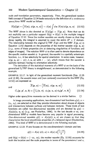
scale and translation parameters, respectively. Then, the generalized random
field concept of Equation 12.34 leads naturally to the definition of a continuous
space/time WRF model as follows

The WRF above is also denoted as X[^](p) = X(p, a). Note that we do
not explicitly use a particular support £t(q) = fi(V>) in the multiple integral
of Equation 12.52. Since the mother wavelets are usually chosen so that they
decay rapidly, the integral is assumed to cover the entire R n x T domain.
The relationship between the original S/TRF X(p) and the WRF X(p, a) in
Equation 12.52 depends on the properties of the mother wavelet t/j(p, u, a)
(e.g., some of these properties aim at detecting singularities of functions and
edges of images). The notation WRF-^> is often used to denote dependence on
the specific mother wavelet ip. In general, the wavelet is a spatially anisotropic
function, i.e., it has selectivity for spatial orientation. In some cases, however,
V>(p, u, a) = i()(r, t, u, a) with r = \s\, which means that the wavelet is
spatially isotropic having no orientation selectivity.
The derivation of the statistical moments of a \NRF-ip on the basis of the
generalized S/TRF theory is straightforward, as demonstrated in the following
example.
EXAMPLE 12.17: In light of the generalized moment functionals (Eqs. 12.35
and 12.36), the wavelet mean and (non-centered) covariance for the WRF (Eq.
12.52) are expressed as

and

Higher order space/time moments can be derived in a similar fashion.
In image processing applications, two-dimensional test functions q(s), s =
(si, 53), are selected so that they provide information about shapes of objects
and intersections between surfaces and between textures. These kinds of test
functions are called two-dimensional wavelets and are denoted by q(s) =
A(a)-^(s, u, a) (e.g., see Poularikas, 1996). In the last decade or so, one-
dimensional WRF-i/) models have become very popular in signal processing.
One-dimensional wavelets q(t) = A(a)ip(t, u, a) are chosen so that they
characterize the local smoothness properties of a temporal signal (Daubechies,
1992). This kind of WRF-f/' is demonstrated in the following example.
EXAMPLE 12.18: If one focuses on the one-dimensional t domain and lets

and Cl(q) = £l(i>) = (-00, oo), the mother wavelet (Eq. 12.55) accounts for
both the location and the scale properties in terms of the parameters t and a,