Page 142 - Neural Network Modeling and Identification of Dynamical Systems

132 4. NEURAL NETWORK BLACK BOX MODELING OF AIRCRAFT CONTROLLED MOTION

the following form:

y(t) = f( y(t − 1), y(t − 2),..., y(t − N y ),
u(t − 1),u(t − 2),...,u(t − N u )), (4.1)

where the value of the output signal y(t) at a
given time instant t is computed using the out-
put values y(t − 1), y(t − 2),..., y(t − N y ) of this
signal for the sequence of the preceding time in-
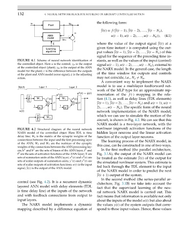
FIGURE 4.1 Scheme of neural network identification of stants, as well as the values of the input (control)
the controlled object. Here u is the control; y p is the output signal u(t − 1),u(t − 2),...,u(t − N u ), external to
of the controlled object (plant); y m is the output of the ANN the NARX model. In the general case, the length
model for the plant; ε is the difference between the outputs
of the plant and ANN model (error signal); ξ is the adjusting of the time window for outputs and controls
action. may not coincide, i.e., N y = N u .
A convenient way to implement the NARX
model is to use a multilayer feedforward net-
work of the MLP type for an approximate rep-
resentation of the f(·) mapping in the rela-
tion (4.1), as well as delay lines (TDL elements)
y(t −1), y(t −2),..., y(t −N y ) and u(t −1),u(t −
2),...,u(t − N u ). The specific form of the neural
network implementation of the NARX model,
which we can use to simulate the motion of the
aircraft, is shown in Fig. 4.2. We can see that this
NARX model is a two-layer network, with the
FIGURE 4.2 Structural diagram of the neural network nonlinear (sigmoid) activation functions of the
NARX model of the controlled object. Here TDL is time hidden layer neurons and the linear activation
delay line; W 1 is the matrix of the synaptic weights of the function of the output layer neurons.
connections between the input and the first processing layer Thelearningprocess of theNARXmodel,in
of the ANN; W 2 and W 3 are the matrices of the synaptic
weights of the connections between the ANN processing lay- this case, can be constructed in one of two ways.
1
2
1
ers; b and b are the sets of biases of the ANN layer; f and In the first method (the parallel architecture,
2
f are the sets of activation functions of the ANN layer; are Fig. 3.1A), the output of the NARX model can
2
1
sets of summation units of the ANN layer; v (t) and v (t) are be treated as the estimate y(t) of the output for
2
1
sets of scalar outputs of summation units; y (t) and y (t) are the simulated nonlinear system. This estimate is
sets of scalar outputs of activation functions; u(t) is the input
signal; y(t) is the output of the ANN model. fed back through the TDL element to the input
of the NARX model in order to predict the next
y(t + 1) output of the system.
In the second method (the series-parallel ar-
control (see Fig. 4.2). It is a recurrent dynamic
chitecture, Fig. 3.1B) we take into account the
layered ANN model with delay elements (TDL
fact that the supervised learning of the neu-
is time delay line) at the inputs of the network ral network NARX model is carried out. This
and with feedback connections from output to fact means that information is available not only
input layers. about the inputs of the model u(t) but also about
The NARX model implements a dynamic the values y(t) of the system outputs that corre-
mapping described by a difference equation of spond to these input values. Hence, these values