Page 74 - Neural Network Modeling and Identification of Dynamical Systems

62 2. DYNAMIC NEURAL NETWORKS: STRUCTURES AND TRAINING METHODS

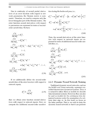
Due to continuity of second partial deriva- ties during the backward pass, i.e.,
tives of an error function with respect to net-
# $
2
L
L

work parameters, the Hessian matrix is sym- δ L,0 = ω i ϕ (n ) − ˜y i − a L ϕ L (n ) ν L,0 ,
L
i
i
i
i
i
i,j
i,j
metric. Therefore, we need to compute only the
l+1
lower-triangular part of the Hessian matrix. The l,0 l l S l+1 l+1,0
error function second derivatives with respect δ i,j = ϕ (n ) w k,i δ k,j
i
i
to parameters are expressed in terms of second- k=1
l+1
order sensitivities. We have l,0 S
l
l
δ
+ ϕ (n )ν i,j w l+1 l+1 ,l = L − 1,...,1.
i
i
k
k,i
k=1
2
∂ E l,m (2.80)
= δ i,k ,
l
∂b ∂b m
i k Then, the second derivatives of the error func-
2
∂ E l,m m−1 tion with respect to network inputs are ex-
= δ i,k a r ,
l
∂b ∂w m pressed in terms of additional second-order sen-
i k,r
2
∂ E l,m l−1 l l−1 l−1 l−1,m sitivities, i.e.,
= δ i,k a j + δ ϕ (n j )ν j,k ,
i j
l
∂w ∂b m S 1
2
i,j k ∂ E 1 1,0
l> 1, ∂a ∂a 0 j = w δ ,
k,i k,j
0
i
2
∂ E 1,1 0 2 k=1
= δ i,k j ∂ E l,0
a ,
1
∂w ∂b 1 = δ ,
i,k
l
i,j k ∂b ∂a 0 k
i
2
∂ E l,m l−1 m−1 2
= δ a a r ∂ E l,0 l−1 l l−1 l−1 l−1,0
l
∂w ∂w m i,k j l 0 = δ a + δ ϕ (n j )ν j,k ,l > 1,
i,k j
i j
i,j k,r ∂w ∂a
i,j k
l
a
+ δ ϕ l−1 (n l−1 )ν l−1,m m−1 ,l > 1, 2
i j j j,k r ∂ E 1,0 0 1
= δ a + δ ,
i
2
1
∂ E 1,1 0 0 ∂w ∂a 0 i,j j
a a .
= δ i,k j r i,j j
1
∂w ∂w 1 2
i,j k,r ∂ E 1,0 0
a ,j = k.
(2.78) 1 0 = δ i,k j
∂w ∂a
i,j k
(2.81)
If we additionally define the second-order
sensitivities of the error function with respect to 2.2.3 Dynamic Neural Network Training
network inputs,
Traditional dynamic neural networks, such as
the NARX and Elman networks, represent con-
trolled discrete time dynamical systems. Thus, it
2
∂ E
l,0
δ , (2.79) is natural to utilize them as models for discrete
i,j l 0
∂n ∂a
i j time dynamical systems. However, they can also
be used as models for the continuous time dy-
namical systems under the assumption of a uni-
then we obtain error function second deriva- form time step t. In this book we focus on
tives with respect to network inputs. First, we the latter problem. That is, we wish to train the
compute the additional second-order sensitivi- dynamic neural network so that it can perform