Page 79 - Neural Network Modeling and Identification of Dynamical Systems

2.3 DYNAMIC NEURAL NETWORK ADAPTATION METHODS 67
line result in a stationary behavior of model • state estimation
states z(t k ) ≡ z(t 0 ), and the corresponding
−
−
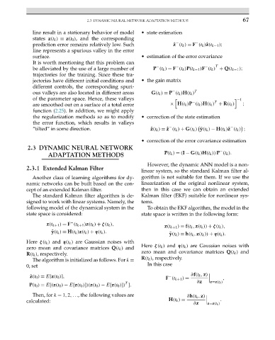
prediction error remains relatively low. Such ˆ z (t k ) = F (t k )ˆz(t k−1 );
line represents a spurious valley in the error
surface. • estimation of the error covariance
It is worth mentioning that this problem can T
−
−
−
be alleviated by the use of a large number of P (t k ) = F (t k )P(t k−1 )F (t k ) + Q(t k−1 );
trajectories for the training. Since these tra-
jectories have different initial conditions and • the gain matrix
different controls, the corresponding spuri-
−
ous valleys are also located in different areas G(t k ) = P (t k )H(t k ) T
of the parameter space. Hence, these valleys T −1
−
are smoothed out on a surface of a total error × H(t k )P (t k )H(t k ) + R(t k ) ;
function (2.25). In addition, we might apply
the regularization methods so as to modify • correction of the state estimation
the error function, which results in valleys

−
“tilted” in some direction. ˆ z(t k ) =ˆz (t k ) + G(t k ) ˜y(t k ) − H(t k )ˆz (t k ) ;
−
• correction of the error covariance estimation
2.3 DYNAMIC NEURAL NETWORK
−
ADAPTATION METHODS P(t k ) = (I − G(t k )H(t k ))P (t k ).
However, the dynamic ANN model is a non-
2.3.1 Extended Kalman Filter
linear system, so the standard Kalman filter al-
Another class of learning algorithms for dy- gorithm is not suitable for them. If we use the
namic networks can be built based on the con- linearization of the original nonlinear system,
cept of an extended Kalman filter. then in this case we can obtain an extended
The standard Kalman filter algorithm is de- Kalman filter (EKF) suitable for nonlinear sys-
signed to work with linear systems. Namely, the tems.
following model of the dynamical system in the To obtain the EKF algorithm, the model in the
state space is considered: state space is written in the following form:
−
z(t k+1 ) = F (t k+1 )z(t k ) + ζ(t k ),
z(t k+1 ) = f(t k ,z(t k )) + ζ(t k ),
˜ y(t k ) = H(t k )z(t k ) + η(t k ).
˜ y(t k ) = h(t k ,z(t k )) + η(t k ).
Here ζ(t k ) and η(t k ) are Gaussian noises with
zero mean and covariance matrices Q(t k ) and Here ζ(t k ) and η(t k ) are Gaussian noises with
R(t k ), respectively. zero mean and covariance matrices Q(t k ) and
R(t k ), respectively.
The algorithm is initialized as follows. For k =
0,set In this case

ˆ z(t 0 ) = E[z(t 0 )], − ∂f(t k ,z)
F (t k+1 ) = ∂z z=z(t k ) ,
T
P(t 0 ) = E[(z(t 0 ) − E[z(t 0 )])(z(t 0 ) − E[z(t 0 )]) ].
Then, for k = 1,2,..., the following values are
∂h(t k ,z)
calculated: H(t k ) = ∂z z=z(t k ) .