Page 115 - Numerical Analysis Using MATLAB and Excel

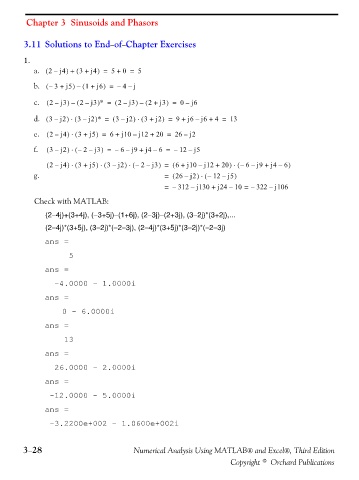
Chapter 3 Sinusoids and Phasors

3.11 Solutions to End−of−Chapter Exercises

1.
a. ( 2 – j4 + ( 3 + j4 = 5 + 0 = 5
)
)
)
)
b. ( – 3 + j5 – ( 1 + j6 = – 4 – j
)
)
c. ( 2 – j3 – ( 2 – j3 ∗ = ( 2 – j3 – ( 2 + j3 = 0 – j6
)
)
)
d. ( 3 – j2 ⋅ ( 3j2 ∗ = ( 3 – j2 ⋅ ( 3 + j2 = 9 + j6 j6 + 4 = 13
)
)
)
–
–
)
e. ( 2 – j4 ⋅ ( 3 + j5 = 6 + j10 – j12 + 20 = 26 j2
)
–
f. ( 3 – j2 ⋅ – ( 2 – j3 = – 6 j9 + j4 – 6 = – 12 j5
)
)
–
–
)
( 2 – j4) ( 3 + j5 ⋅ ) ⋅ ( 3j2 ⋅ – ) – ( 2 – j3 = ( 6 + j10 – j12 + 20 ⋅ – ( 6 – j9 + j4 6 )
)
–
g. = ( 26 – j2 ⋅ – ( 12 – j5 )
)
= – 312 – j130 + j24 – 10 = – 322 – j106
Check with MATLAB:
(2−4j)+(3+4j), (−3+5j)−(1+6j), (2−3j)−(2+3j), (3−2j)*(3+2j),...
(2−4j)*(3+5j), (3−2j)*(−2−3j), (2−4j)*(3+5j)*(3−2j)*(−2−3j)
ans =
5
ans =
-4.0000 - 1.0000i

ans =
0 - 6.0000i

ans =

13
ans =

26.0000 - 2.0000i
ans =

-12.0000 - 5.0000i

ans =
-3.2200e+002 - 1.0600e+002i

3−28 Numerical Analysis Using MATLAB® and Excel®, Third Edition
Copyright © Orchard Publications