Page 110 - Numerical Methods for Chemical Engineering

Problems 99

In the former option, the user supplies a sparse matrix S whose sparsity pattern (location
of nonzero elements) matches that of the Jacobian. That is, even though the Jacobian may
be difficult to compute analytically, the user can at least specify that only a small subset of
Jacobian elements are known to be nonzero. fsolve can use this information to reduce the
computational burden and memory requirement when generating an approximate Jacobian.
With “JacobMult”, the user supplies the name of a routine that returns the product of the
Jacobian matrix with an input vector. The usefulness of this option will become clearer after
our discussion of iterative methods for solving linear algebraic systems in Chapter 6.
fsolve is part of the Optimization Toolkit, and so is not available in all installations of
MATLAB.If fsolve is unavailable, the provided routine reduced Newton.m can be used in
its place. For a single nonlinear algebraic equation, one may also use fzero, that is called
similarly to fsolve,
x = fzero(fun name, x0, Options, P1, P2,...);

Problems

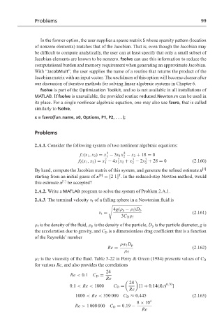
2.A.1. Consider the following system of two nonlinear algebraic equations:

3
2
f 1 (x 1 , x 2 ) = x − 3x 1 x − x 2 + 18 = 0
1
2
3
2
2
2
f 2 (x 1 , x 2 ) = x − 4x x 2 + x − 2x + 28 = 0 (2.160)
1
1
2
2
By hand, compute the Jacobian matrix of this system, and generate the refined estimate x [1]
T
starting from an initial guess of x [0] = [2 1] . In the reduced-step Newton method, would
this estimate x [1] be accepted?
2.A.2. Write a MATLAB program to solve the system of Problem 2.A.1.
2.A.3. The terminal velocity v t of a falling sphere in a Newtonian fluid is
+
4g(ρ p − ρ f )D p
v t = (2.161)
3C D ρ f
ρ f is the density of the fluid, ρ p is the density of the particle, D p is the particle diameter, g is
the acceleration due to gravity, and C D is a dimensionless drag coefficient that is a function
of the Reynolds’ number
ρ f v t D p
Re = (2.162)
µ f
µ f is the viscosity of the fluid. Table 5-22 in Perry & Green (1984) presents values of C D
for various Re, and also provides the correlations
24
Re < 0.1 C D =
Re
24 0.70

0.1 < Re < 1000 C D = [1 + 0.14(Re) ]
Re
1000 < Re < 350 000 C D ≈ 0.445 (2.163)
8 × 10 4
Re > 1 000 000 C D = 0.19 −
Re