Page 106 - Numerical Methods for Chemical Engineering

Bifurcation analysis 95

ircatin int

1 cn
1
di Θ tanent ine

2 2
2 di Θ
n stins

tw stins
1
2
1
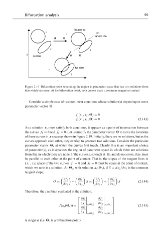
Figure 2.19 Bifurcation point separating the region in parameter space that has two solutions from
that which has none. At the bifurcation point, both curves share a common tangent at contact.

Consider a simple case of two nonlinear equations whose solution(s) depend upon some
parameter vector Θ.

f 1 (x 1 , x 2 ; Θ) = 0
f 2 (x 1 , x 2 ; Θ) = 0 (2.143)

As a solution x s must satisfy both equations, it appears as a point of intersection between
the curves f 1 = 0 and f 2 = 0. Let us modify the parameter vector Θ to move the locations
of these curves in x space as shown in Figure 2.19. Initially, there are no solutions, but as the
curves approach each other, they overlap to generate two solutions. Consider the particular
parameter vector Θ c at which the curves first touch. Clearly this is an important choice
of parameter(s), as it separates the region of parameter space in which there are solutions
from that in which there are none. If the curves just touch at Θ c and do not cross, they must
be parallel to each other at the point of contact. That is, the slopes of the tangent lines in
( x 1 , x 2 ) space of the two curves f 1 = 0 and f 2 = 0 must be equal at the point of contact,
which we note is a solution. At Θ c , with solution x s (Θ c ), if S = dx 2 /dx 1 is the common
tangent slope,

∂ f 1 ∂ f 1 ∂ f 2 ∂ f 2
O = + S = + S (2.144)
∂x 1 ∂x 2 ∂x 1 ∂x 2
Therefore, the Jacobian evaluated at the solution,

 
∂ f 1 ∂ f 1

 ∂x 1 x s (Θ c ) 
J(x s (Θ c )) =  ∂x 2 x s (Θ c )  (2.145)

 ∂ f 2 ∂ f 2 

∂x 1 x s (Θ c ) ∂x 2 x s (Θ c )
is singular (i.e. Θ c is a bifurcation point).