Page 143 - Numerical Methods for Chemical Engineering

132 3 Matrix eigenvalue analysis

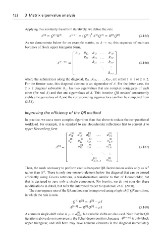
Applying this similarity transform iteratively, we define the rule
[k]
[k]

A [k] = Q [k] R [k] A [k+1] = Q [k] T A Q [k] = R Q [k] (3.165)
As we demonstrate below for an example matrix, as k →∞, this sequence of matrices
becomes of block upper triangular form,
 
R 11 R 12 R 13 ... R 1P
...
R 22 R 23 R 2P
 
 
A [k→∞] =  R 33 ... R 3P  (3.166)


 . . . 
 . . . 
R PP
where the submatrices along the diagonal, R 11 , R 22 ,..., R PP , are either 1 × 1or2 × 2.
For the former case, this diagonal element is an eigenvalue of A. For the latter case, the
2 × 2 diagonal submatrix R jj has two eigenvalues that are complex conjugates of each
other (for real A) and that are eigenvalues of A. This iterative QR method concurrently
yields all eigenvalues of A, and the corresponding eigenvectors can then be computed from
(3.38).

Improving the efficiency of the QR method
In practice, we use a more complex algorithm than that above to reduce the computational
workload. For example, it is standard to use Householder reflections first to convert A to
upper Hessenberg form
 [0] [0] [0] [0] 
a a a ... a
11 12 13 1 N
 [0] [0] [0] [0] 
 a a a ... a 
 21 22 23 2 N 
[0] [0] [0] 

A [0] =  a 32 a 33 ... a 3 N  (3.167)
 
 . . . . . . 
 . . . 
 
[0] [0]
a a
N,N−1 NN
Then, the work necessary to perform each subsequent QR factorization scales only as N 2
3
rather than N . There is only one nonzero element below the diagonal that can be zeroed
efficiently using Givens rotations, a transformation similar to that of Householder, but
that is designed to zero only a single component. For brevity, we do not consider these
modifications in detail, but refer the interested reader to Quateroni et al. (2000).
The convergence rate of the QR method can be improved using single-shift QR iterations,
in which the rule is now
Q [k] R [k] = A [k] − µI
[k]
A [k+1] = R Q [k] + µI (3.168)
[k]
A common single-shift value is µ = a , but variable shifts are also used. Note that the QR
NN
iterations above do not converge to the Schur decomposition, because A [k→∞] is only block
upper triangular, and still have may have nonzero elements in the diagonal immediately