Page 275 - Numerical Methods for Chemical Engineering

264 6 Boundary value problems

1

2
2
1
1

2 1

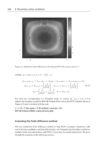
Figure 6.3 Solution by finite differences of the Poisson BVP with a source term f = 1.

scheme, ϕ n = ϕ(x i , y j ), n = (i − 1)N y + j,

ϕ ϕ
A n,n−N y n−N y + A n,n−1 ϕ n−1 + A nn ϕ n + A n,n+1 ϕ n+1 + A n,n+N y n+N y = b n
−1 −1

= A n,n−1 = A n,n+1 = (6.31)
A n,n−N y = A n,n+N y 2 2
( x) ( y)

2 2
A nn = + b n = f (x i , y j )
( x) 2 ( y) 2
For each row corresponding to a boundary point, we merely set A nn = 1, b n = 0to
enforce the boundary condition. BVP 2D Poisson FD.m solves this BVP (solution shown in
Figure 6.3) and is invoked with the code

L=1;H=1;fun name = ‘f rD uniform’; num pts = 51;
BVP 2D Poisson FD(fun name,L,H,num pts);

Extending the finite difference method

We next extend the finite difference method to treat BVPs of greater complexity, with
non-Cartesian coordinates and nonuniform grids, von Neumann-type boundary conditions,
multiple fields, time dependence, and PDEs in more than two spatial dimensions. We do so
through the examples in the following sections.