Page 272 - Numerical Methods for Chemical Engineering

The finite difference method applied to a 2-D BVP 261

B

i 1 i
n 1 n i 1
i1
n
B1

B2
i 1 i 1
n n 1

B

i
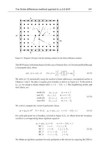
Figure 6.2 Regular 2-D grid with the labeling scheme for the finite difference method.

This BVP arises in fluid mechanics for the case of laminar flow of a Newtonian fluid through
a rectangular duct, where

1 P
ϕ(x, y) = v z (x, y) f (x, y) = − + ρg z (6.13)
µ z
We solve (6.12) numerically using the method of finite differences, encountered earlier in
Chapters 1 and 2. We place a regular grid of points as shown in Figure 6.2. To the point at
(x i , y j ), we assign a unique integer label n = (i − 1)N y + j. The neighboring points, and
their labels, are

north (N) (x i , y j+1 ) m = n + 1
east (E) (x i+1 , y j ) m = n + N y
(6.14)
south (S) (x i , y j−1 ) m = n − 1
west (W) (x i−1 , y j ) m = n − N y

We wish to compute the vector of grid point values,
N
ϕ = [ϕ n ] ∈ N = N x N y ϕ n = ϕ(x i , y j ) n = (i − 1)N y + j (6.15)
For each grid point on a boundary (circled in Figure 6.2), we obtain from the boundary
condition a corresponding linear algebraic equation

ϕ n = ϕ(x i , y j ) = 0 n = (i − 1)N y + j
BC 1 i = 1 1 ≤ j ≤ N y
BC 2 i = N x 1 ≤ j ≤ N y (6.16)
BC 3 1 < i < N x j = 1
BC 4 1 < i < N x j = N y

We obtain an algebraic equation for each grid point in the interior by requiring the PDE to