Page 267 - Numerical Methods for Chemical Engineering

256 5 Numerical optimization

taret
r i
φ deectin ane wind

traectr rectie

taret

r i i
n
θ ee vatin ane
seae ve
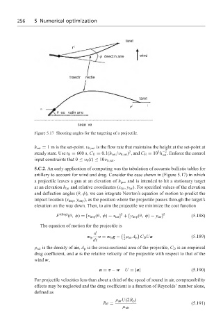
Figure 5.17 Shooting angles for the targeting of a projectile.

h set = 1 m is the set-point. υ 0,set is the flow rate that maintains the height at the set-point at
3 −2
2
steady state. Use t H = 600 s, C U = 0.1(h set /υ 0,set ) , and C H = 10 h . Enforce the control
set
input constraints that 0 ≤ υ 0 (t) ≤ 10υ 0,set .
5.C.2. An early application of computing was the tabulation of accurate ballistic tables for
artillery to account for wind and drag. Consider the case shown in (Figure 5.17) in which
a projectile leaves a gun at an elevation of h gun and is intended to hit a stationary target
at an elevation h tar and relative coordinates (x tar , y tar ). For specified values of the elevation
and deflection angles (θ, φ), we can integrate Newton’s equation of motion to predict the
impact location (x imp , y imp ), as the position where the projectile passes through the target’s
elevation on the way down. Then, to aim the projectile we minimize the cost function
2
F (drag) (θ, φ) = [x imp (θ, φ) − x tar ] + [y imp (θ, φ) − y tar ] 2 (5.188)
The equation of motion for the projectile is
d 1
m p v = m p g − 2 ρ air A p C D Uu (5.189)
dt
ρ air is the density of air, A p is the cross-sectional area of the projectile, C D is an empirical
drag coefficient, and u is the relative velocity of the projectile with respect to that of the
wind w,
u = v − w U =|u| (5.190)

For projectile velocities less than about a third of the speed of sound in air, compressibility
effects may be neglected and the drag coefficient is a function of Reynolds’ number alone,
defined as
ρ air U(2R p )
Re = (5.191)
µ air