Page 265 - Numerical Methods for Chemical Engineering

254 5 Numerical optimization

1

22 22
1
2 22 12
1 22 1
2 2
1 2
22 22
22 1
1 22
2 A
1
22
1
2 2

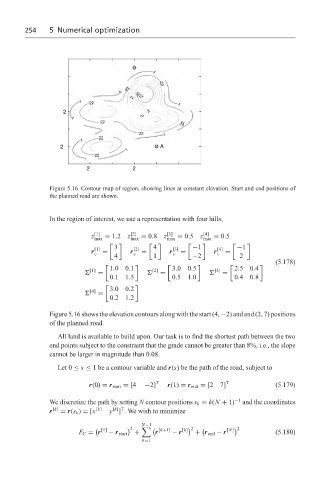
Figure 5.16 Contour map of region, showing lines at constant elevation. Start and end positions of
the planned road are shown.

In the region of interest, we use a representation with four hills,

z [1] = 1.2 z [2] = 0.8 z [3] = 0.5 z [4] = 0.5
max max max max

3 [2] 4 [3] −1 [4] −1
[1]
r = r = r = r =
c c c c
4 1 −2 2
(5.178)

1.00.1 [2] 3.00.5 [3] 2.50.4
[1]
= = =
0.11.5 0.51.0 0.40.8

3.00.2
[4]
=
0.21.2
Figure 5.16 shows the elevation contours along with the start (4, −2) and end (2, 7) positions
of the planned road.
All land is available to build upon. Our task is to find the shortest path between the two
end points subject to the constraint that the grade cannot be greater than 8%, i.e., the slope
cannot be larger in magnitude than 0.08.
Let 0 ≤ s ≤ 1 be a contour variable and r(s) be the path of the road, subject to

r(0) = r start = [4 −2] T r(1) = r end = [27] T (5.179)

We discretize the path by setting N contour positions s k = k(N + 1) −1 and the coordinates
[k] T
r [k] = r(s k ) = [x [k] y ] . We wish to minimize
N−1
2

[1] [k+1] [k] 2 [N] 2
F C = r − r start + r − r + r end − r (5.180)
k=1