Page 264 - Numerical Methods for Chemical Engineering

Problems 253

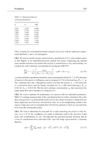
Table 5.2 Measured data of
system performance

θ 1 θ 2 F(θ)
2.653 2.639 0.948
2.625 2.703 0.744
1.865 2.699 0.381
2.591 3.104 0.393
1.337 2.772 0.648
1.779 2.699 0.411
2.470 2.515 1.162
1.265 3.247 0.784

Then, compute the constrained minimum along the unit circle with the additional require-
ments that both x 1 and x 2 be nonnegative.

5.B.1. We wish to use the enzyme whose kinetics, described by (5.51), were studied earlier
in this chapter, in an immobilized-enzyme packed bed reactor. Neglecting any internal
mass transfer resistance (we assume the enzyme is immobilized in very small pellets), we
compute the outlet substrate concentration by solving the ODE-IVP

dc S 1 V m c S
=− c S (W = 0) = c S0 (5.176)
dW α c υ K m + c S + K −1 2
c
si S
−4
c S0 is the substrate concentration in moles, and is constrained to lie in [10 , 2]. W is the mass
of enzyme in the reactor in milligrams, and we integrate (5.176) to the total mass W R = 1g.
6
The volumetric flow rate v through the reactor is in liters per minute. α c = 10 µmol/mol
is a conversion factor, and the kinetic constants are V m = 200 µmol/(min mg E ), K m =
0.201 M, K si = 0.5616 M. Plot the inlet substrate concentration c S0 that maximizes the
outlet molar flow rate of product, as a function of υ.
5.B.2. We wish to optimize the performance of a process with two adjustable parameters.
Table 5.2 contains measured data of the cost function that we wish to minimize. Fit to this
data some general ( e.g. polynomial) model and use this model to propose a design that you
think might have an even lower cost function value. To avoid extrapolating outside of the
region of data, use a set of constraints that will limit the amount to which we can search far
away from the existing data points.
5.B.3. We wish to determine the best path for a road connecting two points in hilly ter-
2
rain. Let r ∈ be the coordinates of a point in kilometers and let the elevation at that
point, also in kilometers, be z(r). We represent the measured ground elevation data as
a sum of contributions from individual hills, each hill being represented by a Gaussian
function,

N h
−1
[k] 1 [k] [k]
z(r) = z exp − r − r c · [k] r − r c (5.177)
max 2
k=1