Page 259 - Numerical Methods for Chemical Engineering

248 5 Numerical optimization

a 2

2
t
1

1
2 1
t

2
t
1

2 1
t
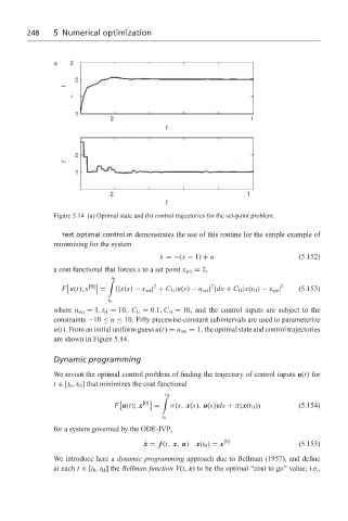
Figure 5.14 (a) Optimal state and (b) control trajectories for the set-point problem.

test optimal control.m demonstrates the use of this routine for the simple example of
minimizing for the system

˙ x =−(x − 1) + u (5.152)
a cost functional that forces x to a set point x set = 2,

[0] t H ' 2 2 2
F u(t); x = {|x(s) − x set | + C U |u(s) − u set | }ds + C H |x(t H ) − x set | (5.153)
t 0
where u set = 1, t H = 10, C U = 0.1, C H = 10, and the control inputs are subject to the
constraints −10 ≤ u ≤ 10. Fifty piecewise-constant subintervals are used to parameterize
u(t). From an initial uniform guess u(t) = u set = 1, the optimal state and control trajectories
are shown in Figure 5.14.

Dynamic programming
We revisit the optimal control problem of finding the trajectory of control inputs u(t) for
t ∈ [t 0 , t H ] that minimizes the cost functional

[0] t H '
F u(t); x = σ(s, x(s), u(s))ds + π(x(t H )) (5.154)
t 0
for a system governed by the ODE-IVP,

˙ x = f (t, x, u) x(t 0 ) = x [0] (5.155)
We introduce here a dynamic programming approach due to Bellman (1957), and define
at each t ∈ [t 0 , t H ] the Bellman function V(t, x) to be the optimal “cost to go” value; i.e.,