Page 255 - Numerical Methods for Chemical Engineering

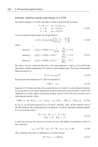
244 5 Numerical optimization

Example. Optimal steady-state design of a CSTR

We wish to design a 1-l CSTR to produce C from A and B by the reactions
A + B → C r R1 = k 1 (T )c A c B
(5.129)
A → S 1 r R2 = k 2 (T )c A
C → S 2 r R3 = k 3 (T )c C
The rate constants depend upon the temperature as
1
E a j T ref
k j (T ) = k j (T ref )exp 1 − (5.130)
RT ref T
where
l E a1
reaction 1 k 1 (T ref = 298 K) = 2.3 = 15.4
mol h RT ref
E a2
−1
reaction 2 k 2 (T ref = 298 K) = 0.2h = 17.9 (5.131)
RT ref
reaction 3 k 3 (T ref = 298 K) = 0.1h −1 E a3 = 22.3
RT ref
We wish to vary the volumetric flow rate v, the concentrations c A0 and c B0 of A and B in the
inlet stream, and the temperature T to achieve various design goals. The vector of adjustable
design parameters is
θ = [υ c A0 c B0 T ] T (5.132)

To maximize the production of C, the cost function is
(5.133)
F 1 (θ) =−υc C
Equation (5.133) does not take into account the loss of A and C to side product formation.
Let us say that we can easily separate the products and recycle the unreacted A and B. For
simplicity, let us also neglect any heating/cooling or power costs. The net economic cost of
operating the reactor is then
c ] (5.134)
F 2 (θ) = (−υ)[−$ A (c A0 − c A ) − $ B (c B0 − c B ) + $ C c C − $D S 1 S 1
c − $D S 2 S 2
are the disposal costs of
$ A , $ B , $ C are the prices per mole of A, B, and C, and $D S 1 , $D S 2
the side products. By minimizing this cost function, we get the maximal economic benefit.
Let us assume the prices

$ A = 4.5$ B = 1.1$ C = 8.2
(5.135)
= 1.0
$D S 1 = 1.0$D S 2
A and B are fed into the reactor in a carrier solvent, with initial concentrations subject to
the constraints

c A0 ≥ 10 −4 M c B0 ≥ 10 −4 M c A0 + c B0 ≤ 2 M (5.136)
The volumetric flow rate is constrained to be in the interval

10 −4 l/h ≤ υ ≤ 360l/h (5.137)