Page 257 - Numerical Methods for Chemical Engineering

246 5 Numerical optimization

M
u(t) ∈ is a set of tunable control inputs and θ is a set of fixed system parameters.
For simplicity, we drop explicit reference to the latter and write the ODE system as ˙x =
[0]
f (t, x, u). At time t 0 , we start at the initial state x(t 0 ) = x , and wish to determine the
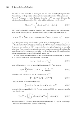
trajectory of control inputs u(t) within t ∈ [t 0 , t H ] that minimize a cost functional

[0] t H '
F u(t); x = σ(s, x(s), u(s))ds + π(x(t H )) (5.144)
t 0
t H is the horizon time for this optimal control problem. For example, we may wish to maintain
the system at some set point x set , in which case a suitable choice of cost functional is

[0] t H ' 2 2 2
F u(t); x = {|x(s) − x set | + C U |u(s) − u set | }ds + C H |x(t H ) − x set | (5.145)
t 0
u set is the input necessary to maintain the system steady at the set point and C U , C H > 0.
How do we find the “best” u(t) that minimizes (5.144)? We describe first a direct approach
for an open-loop problem in which we compute the entire optimal trajectory for a specific
initial state. Then, we outline an alternative dynamic programming approach that turns the
integral equation (5.144) into a corresponding time-dependent partial differential equation,
and generates a closed-loop optimal feedback control law.
As a first approach, let us parameterize u(t) as a piecewise-constant function by splitting
[t 0 , t H ] into N S subintervals separated by the time points
t H − t 0
t k = t 0 + k( t) t = (5.146)
N S
[k]
In the subinterval t k−1 ≤ t < t k , we hold u(t) constant at u . Thus, we write
N s
[k] 1, t k−1 ≤ t < t k
u(t) = u k (t) k (t) = (5.147)
0, otherwise
k=1
N S M
and characterize the trajectory u(t) by the vector U ∈ ,
T [1] T [2] T [N s ] T

U = u u ... u (5.148)
Let x(t; U) be the solution to the ODE-IVP
d [0]
x(t; U) = f (t, x(t; U), u(t; U)) x(t 0 ) = x (5.149)
dt
where u(t; U) is computed by (5.147). The cost functional (5.144) then is approximated by
a cost function of U,
 
N s t k '

[0] [k]
F U; x =  σ s, x(s; U), u ds  + π(x(t H ; U)) (5.150)
k=1
t k−1
We then minimize (5.150) using the techniques described above. As U can be of quite high
a dimension, this optimization problem can be costly.