Page 283 - Numerical Methods for Chemical Engineering
P. 283

272     6 Boundary value problems


                       1

                                                     e     1  e   1
                    ϕ                          ϕ       c
                            e  c    1   e   1   2
                                           1                          1

                                                 1
                         e  c    1   e              e  c    21   e   11
                    ϕ                          ϕ
                     2
                                           1                          1

                       1                         1
                          e  c       e   2         e  c    1   e   1
                    ϕ                          ϕ
                                               −
                                           1                          1

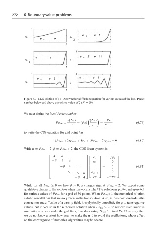
                   Figure 6.7 CDS solution of a 1-D convection/diffusion equation for various values of the local Peclet
                   number below and above the critical value of 2 (N = 50).


                   We next define the local Peclet number
                                            v( z)         ( z)      Pe
                                     Pe loc ≡     = (Pe)        =                     (6.79)
                                                           L      N + 1

                   to write the CDS equation for grid point j as

                                   − (Pe loc + 2)ϕ j−1 + 4ϕ j + (Pe loc − 2)ϕ j+1 = 0  (6.80)

                   With α ≡ Pe loc − 2,β ≡ Pe loc + 2, the CDS linear system is

                                    4    α                             
                                                      
                                                            ϕ 1       βϕ 0
                                  −β    4   α         
                                                         ϕ 2      0  
                                                 .                     
                                                 .        .       .  
                                       −β   4     .       . .   =   . .         (6.81)
                                                      
                                             .   .                     
                                             .   .                0  
                                             .    .  α    ϕ N−1
                                                 −β   4     ϕ N      −αϕ 1
                   While for all Pe loc ≥ 0wehave β> 0, α changes sign at Pe loc = 2. We expect some
                   qualitative change in the solution when this occurs. The CDS solution is plotted in Figure 6.7
                   for various values of Pe loc for a grid of 50 points. When Pe loc >2, the numerical solution
                   exhibits oscillations that are not present in the true solution. Also, as this equation models the
                   convection and diffusion of a density field, it is physically unrealistic for ϕ to take negative
                   values, but it does so in the numerical solution when Pe loc > 2. To remove such spurious
                   oscillations, we can make the grid finer, thus decreasing Pe loc for fixed Pe. However, often
                   we do not know a priori how small to make the grid to avoid the oscillations, whose effect
                   on the convergence of numerical algorithms may be severe.
   278   279   280   281   282   283   284   285   286   287   288