Page 137 -

120 3. Finite Element Methods for Linear Elliptic Problems

conv{x,a ,a }
3
2
.
a . a
3 2
.
x

conv{a ,x,a } conv{a ,a ,x}
.
1 3 1 2
a
1
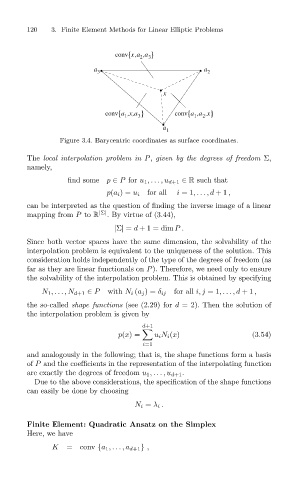
Figure 3.4. Barycentric coordinates as surface coordinates.

The local interpolation problem in P, given by the degrees of freedom Σ,
namely,
find some p ∈ P for u 1 ,... ,u d+1 ∈ R such that
for all i =1,... ,d +1 ,
p(a i )= u i
can be interpreted as the question of finding the inverse image of a linear
mapping from P to R |Σ| . By virtue of (3.44),
|Σ| = d +1 = dim P.
Since both vector spaces have the same dimension, the solvability of the
interpolation problem is equivalent to the uniqueness of the solution. This
consideration holds independently of the type of the degrees of freedom (as
far as they are linear functionals on P). Therefore, we need only to ensure
the solvability of the interpolation problem. This is obtained by specifying

N 1 ,... ,N d+1 ∈ P with N i (a j )= δ ij for all i, j =1,...,d +1 ,
the so-called shape functions (see (2.29) for d = 2). Then the solution of
the interpolation problem is given by
d+1

p(x)= u i N i (x) (3.54)
i=1
and analogously in the following; that is, the shape functions form a basis
of P and the coefficients in the representation of the interpolating function
are exactly the degrees of freedom u 1 ,...,u d+1.
Due to the above considerations, the specification of the shape functions
can easily be done by choosing
N i = λ i .

Finite Element: Quadratic Ansatz on the Simplex
Here, we have
K =conv {a 1 ,... ,a d+1 } ,