Page 133 -

116 3. Finite Element Methods for Linear Elliptic Problems

As in the example of (2.27) (cf. Lemma 2.10), V h is defined by specifying
P K and the degrees of freedom on K for K ∈T h . These have to be chosen
such that, on the one hand, they enforce the continuity of v ∈ V h and,
on the other hand, the satisfaction of the homogeneous Dirichlet bound-
ary conditions at the nodes. For this purpose, compatibility between the
Dirichlet boundary condition and the triangulation is necessary, since it
will be required in (T6).
As can be seen from the proof of Lemma 2.10, it is essential
that the interpolation problem, locally defined on K ∈
(F1) (3.41)
T h by the degrees of freedom, is uniquely solvable in P K ,
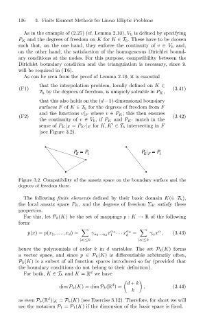
that this also holds on the (d−1)-dimensional boundary
surfaces F of K ∈T h for the degrees of freedom from F
and the functions v| F where v ∈ P K ; this then ensures
(F2) (3.42)
the continuity of v ∈ V h ,if P K and P K matchinthe
sense of P K | F = P K | F for K, K ∈T h intersecting in F

(see Figure 3.2).
. .
P = P P = P
K 1 K F 1
.
. .

Figure 3.2. Compatibility of the ansatz space on the boundary surface and the
degrees of freedom there.

The following finite elements defined by their basic domain K(∈T h ),
the local ansatz space P K , and the degrees of freedom Σ K satisfy these
properties.
For this, let P k (K) be the set of mappings p : K → R of the following
form:
α
x
p(x)= p(x 1 ,...,x d )= γ α 1 ...α d 1 α 1 ··· x α d = γ α x , (3.43)
d
|α|≤k |α|≤k
hence the polynomials of order k in d variables. The set P k (K)forms
a vector space, and since p ∈P k (K) is differentiable arbitrarily often,
P k (K) is a subset of all function spaces introduced so far (provided that
the boundary conditions do not belong to their definition).
d
For both, K ∈T h and K = R we have

d + k
d
dim P k (K)= dim P k (R )= , (3.44)
k
d
as even P k (R )| K = P k (K) (see Exercise 3.12). Therefore, for short we will
use the notation P 1 = P 1 (K) if the dimension of the basic space is fixed.