Page 339 -

322 7. Discretization of Parabolic Problems

reflecting the exponential decay. For example, for Θ = 1, the (error in the)
initial data is damped with the factor
1
n
n
E h,τ = R(−λ min τ) = ,
h
(1 + λ min τ) n
which for τ ≤ τ 0 for some fixed τ 0 > 0 can be estimated by
exp(−λnτ) for some λ> 0.

We conclude this section with an example.
1
Example 7.27 (Prothero-Robinson model) Let g ∈ C [0,T ]be given.
We consider the initial value problem

ξ + λ(ξ − g)= g , t ∈ (0,T ) ,
ξ(0) = ξ 0 .
Obviously, g is a particular solution of the differential equation, so the
general solution is

ξ(t)= e −λt [ξ 0 − g(0)] + g(t) .

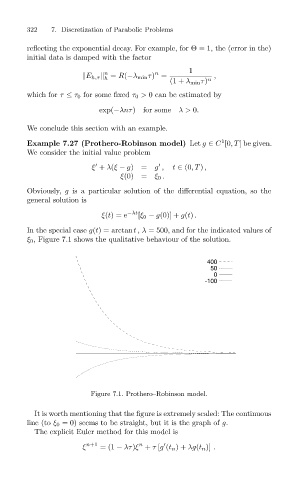
In the special case g(t) = arctant, λ = 500, and for the indicated values of
ξ 0 , Figure 7.1 shows the qualitative behaviour of the solution.

400
50
0
-100

Figure 7.1. Prothero–Robinson model.

It is worth mentioning that the figure is extremely scaled: The continuous
line (to ξ 0 = 0) seems to be straight, but it is the graph of g.
The explicit Euler method for this model is
n

ξ n+1 =(1 − λτ)ξ + τ [g (t n )+ λg(t n )] .