Page 73 -

56 2. Finite Element Method for Poisson Equation

This approach is called the Galerkin method. Or solve instead of (2.22) the
finite-dimensional minimization problem,

find u h ∈ V h with F(u h)= min F(v) v ∈ V h . (2.24)
This approach is called the Ritz method.
It is clear from Lemma 2.3 and Remark 2.4 that the Galerkin method
and the Ritz method are equivalent for a positive and symmetric bilinear
form. The finite-dimensional subspace V h is called an ansatz space.
The finite element method can be interpreted as a Galerkin method (and
in our example as a Ritz method, too) for an ansatz space with special
properties. In the following, these properties will be extracted by means of
the simplest example.
1
Let V be defined by (2.7) or let V = H (Ω).
0
The weak formulation of the boundary value problem (2.1), (2.2)
corresponds to the choice

a(u, v):= ∇u ·∇vdx , b(v):= fv dx .
Ω Ω
2
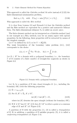
Let Ω ⊂ R be a domain with a polygonal boundary; i.e., the boundary
Γ of Ω consists of a finite number of straight-line segments as shown in
Figure 2.2.

Ω

Figure 2.2. Domain with a polygonal boundary.

Let T h be a partition of Ω into closed triangles K (i.e., including the
boundary ∂K) with the following properties:

K;
(1) Ω= ∪ K∈T h

(2) For K, K ∈T h ,K = K ,

int (K) ∩ int (K )= ∅ , (2.25)
where int (K) denotes the open triangle (without the boundary ∂K).

(3) If K = K but K ∩K = ∅,then K ∩K is either a point or a common

edge of K and K (cf. Figure 2.3).

A partition of Ω with the properties (1), (2) is called a triangulation
of Ω. If, in addition, a partition of Ω satisfies property (3), it is called a
conforming triangulation (cf. Figure 2.4).