Page 102 - Numerical methods for chemical engineering

88 2 Nonlinear algebraic systems

a 1 1

2 2
2 −1 − 1
v s τ a × 1
c 1 d 1

2 2

1 2 1 1
searr ate s −1 viscsit a s
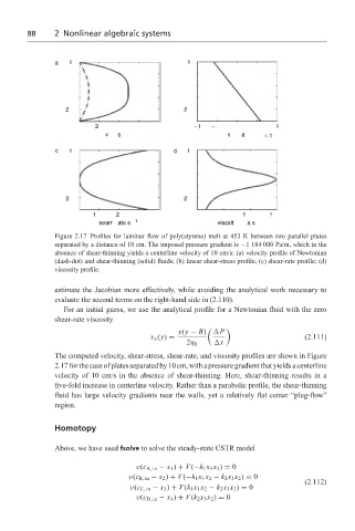
Figure 2.17 Profiles for laminar flow of poly(styrene) melt at 453 K between two parallel plates
separated by a distance of 10 cm. The imposed pressure gradient is −1 184 000 Pa/m, which in the
absence of shear-thinning yields a centerline velocity of 10 cm/s: (a) velocity profile of Newtonian
(dash-dot) and shear-thinning (solid) fluids; (b) linear shear-stress profile; (c) shear-rate profile; (d)
viscosity profile.

estimate the Jacobian more effectively, while avoiding the analytical work necessary to
evaluate the second terms on the right-hand side in (2.110).
For an initial guess, we use the analytical profile for a Newtonian fluid with the zero
shear-rate viscosity

y(y − B) P
v x (y) = (2.111)
2η 0 x
The computed velocity, shear-stress, shear-rate, and viscosity profiles are shown in Figure
2.17 for the case of plates separated by 10 cm, with a pressure gradient that yields a centerline
velocity of 10 cm/s in the absence of shear-thinning. Here, shear-thinning results in a
five-fold increase in centerline velocity. Rather than a parabolic profile, the shear-thinning
fluid has large velocity gradients near the walls, yet a relatively flat center “plug-flow”
region.

Homotopy

Above, we have used fsolve to solve the steady-state CSTR model

υ(c A, in − x 1 ) + V (−k 1 x 1 x 2 ) = 0
υ(c B, in − x 2 ) + V (−k 1 x 1 x 2 − k 2 x 3 x 2 ) = 0
(2.112)
υ(c C, in − x 3 ) + V (k 1 x 1 x 2 − k 2 x 3 x 2 ) = 0
υ(c D, in − x 4 ) + V (k 2 x 3 x 2 ) = 0