Page 98 - Numerical methods for chemical engineering

84 2 Nonlinear algebraic systems

fsolve is unavailable. For further information on the use of reduced Newton.m, consult
the help section at the beginning of that file.
The syntax for using fsolve to find an approximate solution x and its function value f
(near zero) is

[x, f] = fsolve(fun name, x0, Options, P1, P2, . . . );
fun name is the name of the function that returns the function vector,

f = fun name(x, P1, P2, . . . );
or, if optionally it returns the Jacobian matrix as well,

[f, Jac] = fun name(x, P1, P2, . . . );

P1, P2,... are optional parameters passed through fsolve. x0 is the initial guess. Options is a
data structure managed by the command optimset that allows us to modify the performance
of fsolve. Unless the number of equations is very large, it is best to start with
Options = optimset(‘LargeScale’, ‘off’);

We then can add additional fields to override the default options (type help optimset for
further details). For example, if your routine returns as a second argument the Jacobian
matrix evaluated at x, let fsolve know this by

Options = optimset(Options, ‘Jacobian’, ‘on’);

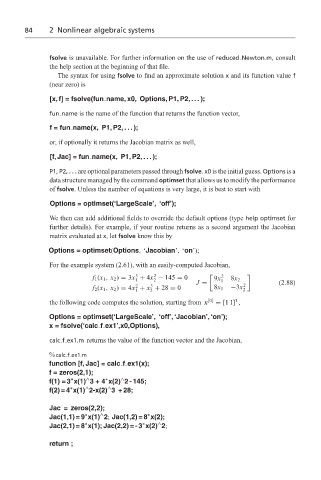
For the example system (2.61), with an easily-computed Jacobian,
3
2
f 1 (x 1 , x 2 ) = 3x + 4x − 145 = 0 9x 2
1 2 J = 1 8x 2 (2.88)
2
3
f 2 (x 1 , x 2 ) = 4x + x + 28 = 0 8x 1 −3x 2
1 2 2
T
the following code computes the solution, starting from x [0] = [1 1] ,
Options = optimset(‘LargeScale’, ‘off’, ‘Jacobian’, ‘on’);
x = fsolve(‘calc f ex1’,x0,Options),
calc f ex1.m returns the value of the function vector and the Jacobian,
% calc f ex1.m
function [f, Jac] = calc f ex1(x);
f = zeros(2,1);
∧
∗
∗
f(1) = 3 x(1) 3+4 x(2) 2 - 145;
∧
∧
∗
f(2) = 4 x(1) 2-x(2) 3 + 28;
∧
Jac = zeros(2,2);
∗
∧
∗
Jac(1,1) = 9 x(1) 2; Jac(1,2) = 8 x(2);
∗
∧
∗
Jac(2,1) = 8 x(1); Jac(2,2) = - 3 x(2) 2;
return ;