Page 132 - Numerical methods for chemical engineering

118 3 Matrix eigenvalue analysis

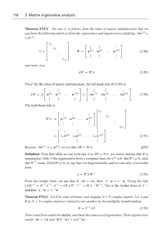
Theorem EVG2 For any A, it follows from the rules of matrix multiplication that we
can form the following matrices from the eigenvalues and eigenvectors satisfying Aw [ j] =
[ j]
λ j w ,
 
λ 1
 
| | |
λ 2
 
  w [1] w [2] ... w (3.88)
. .  W =  [N] 
= 
 . 
| | |
λ N
and write A as
AW = W (3.89)
Proof By the rules of matrix multiplication, the left-hand side of (3.89) is
   
| | | | | |
AW = A  w [1] w [2] ... w [N]  =  Aw [1] Aw [2] ... Aw [N]  (3.90)
| | | | | |
The right-hand side is
 
λ 1
 
| | |
 λ 2 
W =  w [1] w [2] ... w [N]   
 . . 
 . 
| | |
λ N
 
| | |
=  λ 1 w [1] λ 2 w [2] ... λ N w [N]  (3.91)
| | |
[ j]
Because Aw [ j] = λ j w , we see that AW = W . QED
Definition Note that while we can write any A as AW = W ,we cannot assume that W is
N
nonsingular. Only if the eigenvectors form a complete basis for C will det(W) = 0, such
that W −1 exists. If det(W) = 0, we say that A is diagonalizable, and we can write A in Jordan
form,

A = W W −1 (3.92)
−1
−1
From the Jordan form, we see that if Aw = λw, then A w = λ w. Using the rule
−1
−1
−1
)
(AB) −1 = B −1 A , A −1 = (W W −1 −1 = W W −1 . This is the Jordan form of A ,
−1
−1
and thus A w = λ w.
Theorem EVG3 Let S be some arbitrary non singular N × N complex matrix. Let A and
BbeN × N complex matrices related to one another by the similarity transformation
B = S −1 AS (3.93)
Then A and B are said to be similar, and share the same set of eigenvalues. Their eigenvectors
−1
−1
satisfy Aw = λw and B(S w) = λ(S w).