Page 24 - Numerical methods for chemical engineering

10 1 Linear algebra

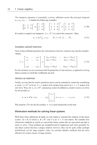
The transpose operation is essentially a mirror reflection across the principal diagonal
a 11 , a 22 , a 33 ,.... Consider the following examples:
T
    
T 14 123 147

123
=  25   456  =  258  (1.50)
456
36 789 369
T
If a matrix is equal to its transpose, A = A , it is said to be symmetric. Then,
T
a ij = A = a ji ∀i, j ∈{1, 2,..., N} (1.51)
ij

Complex-valued matrices
Here we have defined operations for real matrices; however, matrices may also be complex-
valued,
   
c 11 ... c 1N (a 11 + ib 21 ) ... (a 1N + ib 1N )
... (a 21 + ib 21 ) ... (a 2N + ib 2N )
c 21 c 2N
   

C =  .   . .  (1.52)
 . . .  =  . . . . 
.


. 
(a M1 + ib M1 ) ... (a MN + ib MN )
c M1 ... c MN
For the moment, we are concerned with the properties of real matrices, as applied to solving
linear systems in which the coefficients are real.
Vectors as matrices
Finally, we note that the matrix operations above can be extended to vectors by considering
N
a vector v ∈ to be an N × 1 matrix if in column form and to be a 1 × N matrix if in
N
row form. Thus, for v, w ∈ , expressing vectors by default as column vectors, we write
the dot product as
 
w 1
T  . 
.
v · w = v w = [v 1 ··· v N ]  .  = v 1 w 1 +· · · + v N w N (1.53)
w N
T
The notation v w for the dot product v · w is used extensively in this text.
Elimination methods for solving linear systems

With these basic definitions in hand, we now begin to consider the solution of the linear
N
system Ax = b, in which x, b ∈ and A is an N × N real matrix. We consider here
elimination methods in which we convert the linear system into an equivalent one that is
easier to solve. These methods are straightforward to implement and work generally for
any linear system that has a unique solution; however, they can be quite costly (perhaps
prohibitively so) for large systems. Later, we consider iterative methods that are more
effective for certain classes of large systems.