Page 39 - Numerical methods for chemical engineering

Existence and uniqueness of solutions 25

ℜ
ℜ B A ℜ
w v Bw Av ABw

AB
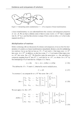
Figure 1.3 Interpreting matrix multiplication C = AB as sequence of linear transformations.

a linear transformation, we can understand better the existence and uniqueness properties
N
of Ax = b. We see that a solution exists if there is some vector x ∈ that is mapped
N
into b ∈ by A, and that this solution is unique if there exists no other y = x that is also
mapped into b by A.

Multiplication of matrices
Before continuing with our discussion of existence and uniqueness, let us see how the inter-
pretation of a matrix as a linear transformation immediately dictates a rule for multiplying
P
two matrices. Let us say that we have an M × P real matrix A that maps every v ∈
M
into some Av ∈ . In addition, we also have some P × N real matrix B that maps every
N
P
w ∈ into some Bw ∈ . We therefore make the association v = Bw and define a
N M N M
composite mapping from into , C, such that for w ∈ , we obtain Cw ∈ by
first multiplying w by B and then by A (Figure 1.3). That is,
v = Bw Cw = Av = A(Bw) = (AB)w (1.126)
This defines the M × N matrix C, obtained by matrix multiplication,

C = AB (1.127)

N
P
To construct C, we compute for w ∈ the vector Bw ∈ ,
 
N

   
b 11 b 12 ... b 1N w 1 b 1 j w j 

 j=1
... 
b 21 b 22 b 2N w 2
   
 . 

 

Bw =  . . .   .  =  .  (1.128)
 . .  . 
.
.
.
.
.   . 
N 

 
b P1 b P2 ... b PN w N b Pj w j
j=1
P
We next apply A to Bw ∈ ,
N  P N 
 

 
a 11 a 12 ... a 1P b 1 j w j  a 1k b kj w j

 j=1  j=1 
...   k=1
a 21 a 22 a 2P
  
 .  .

A(Bw) =  . .   .   . 
 . . .   .  =  . 
.
.
.
. 
N   P N 

   
a M1 a M2 ... a MP b Pj w j a Mk b kj w j
j=1 k=1 j=1
(1.129)