Page 80 - Numerical methods for chemical engineering

66 2 Nonlinear algebraic systems

stin at 1 stin at
2

2

stin at 2

1 1 2 2

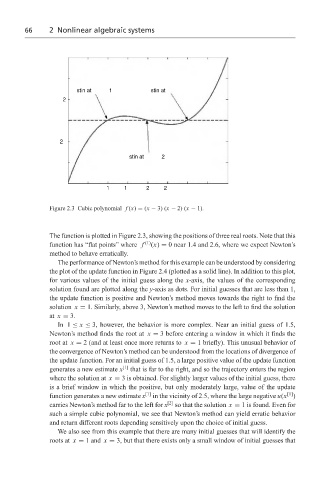
Figure 2.3 Cubic polynomial f (x) = (x − 3) (x − 2) (x − 1).

The function is plotted in Figure 2.3, showing the positions of three real roots. Note that this
function has “flat points” where f (1) (x) = 0 near 1.4 and 2.6, where we expect Newton’s
method to behave erratically.
The performance of Newton’s method for this example can be understood by considering
the plot of the update function in Figure 2.4 (plotted as a solid line). In addition to this plot,
for various values of the initial guess along the x-axis, the values of the corresponding
solution found are plotted along the y-axis as dots. For initial guesses that are less than 1,
the update function is positive and Newton’s method moves towards the right to find the
solution x = 1. Similarly, above 3, Newton’s method moves to the left to find the solution
at x = 3.
In 1 ≤ x ≤ 3, however, the behavior is more complex. Near an initial guess of 1.5,
Newton’s method finds the root at x = 3 before entering a window in which it finds the
root at x = 2 (and at least once more returns to x = 1 briefly). This unusual behavior of
the convergence of Newton’s method can be understood from the locations of divergence of
the update function. For an initial guess of 1.5, a large positive value of the update function
generates a new estimate x [1] that is far to the right, and so the trajectory enters the region
where the solution at x = 3 is obtained. For slightly larger values of the initial guess, there
is a brief window in which the positive, but only moderately large, value of the update
[1]
function generates a new estimate x [1] in the vicinity of 2.5, where the large negative u(x )
carries Newton’s method far to the left for x [2] so that the solution x = 1 is found. Even for
such a simple cubic polynomial, we see that Newton’s method can yield erratic behavior
and return different roots depending sensitively upon the choice of initial guess.
We also see from this example that there are many initial guesses that will identify the
roots at x = 1 and x = 3, but that there exists only a small window of initial guesses that