Page 78 - Numerical methods for chemical engineering

64 2 Nonlinear algebraic systems

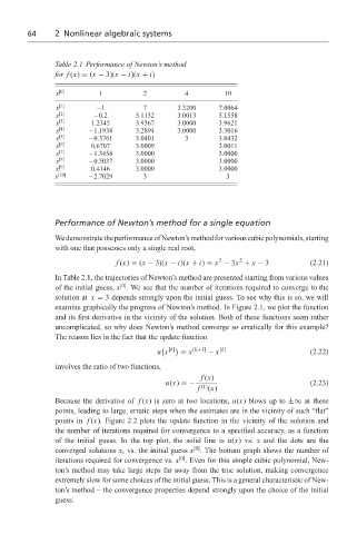
Table 2.1 Performance of Newton’s method
for f (x) = (x − 3)(x − i)(x + i)

x [0] 1 2 4 10
x [1] −1 7 3.3200 7.0064
x [2] −0.2 5.1132 3.0013 5.1558
x [3] 1.2345 3.9367 3.0000 3.9621
x [4] −1.1938 3.2894 3.0000 3.3016
x [5] −0.3761 3.0401 3 3.0432
x [6] 0.6707 3.0009 3.0011
x [7] −1.3458 3.0000 3.0000
x [8] −0.5037 3.0000 3.0000
x [9] 0.4146 3.0000 3.0000
x [10] −2.7029 3 3

Performance of Newton’s method for a single equation
WedemonstratetheperformanceofNewton’smethodforvariouscubicpolynomials,starting
with one that possesses only a single real root,
2
3
f (x) = (x − 3)(x − i)(x + i) = x − 3x + x − 3 (2.21)
In Table 2.1, the trajectories of Newton’s method are presented starting from various values
[0]
of the initial guess, x . We see that the number of iterations required to converge to the
solution at x = 3 depends strongly upon the initial guess. To see why this is so, we will
examine graphically the progress of Newton’s method. In Figure 2.1, we plot the function
and its first derivative in the vicinity of the solution. Both of these functions seem rather
uncomplicated, so why does Newton’s method converge so erratically for this example?
The reason lies in the fact that the update function
[k] [k+1] [k]
u x = x − x (2.22)
involves the ratio of two functions,
f (x)
u(x) =− (1) (2.23)
f (x)
Because the derivative of f (x) is zero at two locations, u(x) blows up to ±∞ at these
points, leading to large, erratic steps when the estimates are in the vicinity of such “flat”
points in f (x). Figure 2.2 plots the update function in the vicinity of the solution and
the number of iterations required for convergence to a specified accuracy, as a function
of the initial guess. In the top plot, the solid line is u(x) vs. x and the dots are the
[0]
converged solutions x s vs. the initial guess x . The bottom graph shows the number of
[0]
iterations required for convergence vs. x . Even for this simple cubic polynomial, New-
ton’s method may take large steps far away from the true solution, making convergence
extremely slow for some choices of the initial guess. This is a general characteristic of New-
ton’s method – the convergence properties depend strongly upon the choice of the initial
guess.