Page 73 - Numerical methods for chemical engineering

Problems 59

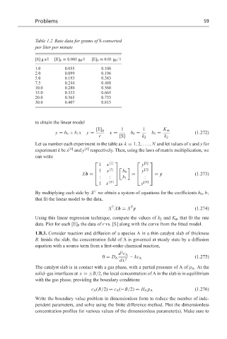
Table 1.2 Rate data for grams of S converted
per liter per minute

[S] g s/l [E] 0 = 0.005 g E /l [E] 0 = 0.01 g E /l
1.0 0.055 0.108
2.0 0.099 0.196
5.0 0.193 0.383
7.5 0.244 0.488
10.0 0.280 0.560
15.0 0.333 0.665
20.0 0.365 0.733
30.0 0.407 0.815

to obtain the linear model
[E] 0 1 1 K m
y = b 0 + b 1 x y = x = b 0 = b 1 = (1.272)
r [S] k 2 k 2
Let us number each experiment in the table as k = 1, 2,..., N and let values of x and y for
experiment k be x [k] and y [k] respectively. Then, using the laws of matrix multiplication, we
can write
 [1]   [1] 
1 x y

1 x [2]  y [2] 
 b 0 
Xb =   =   = y (1.273)
 : :  b 1  : 
1 x [N] y [N]
T
By multiplying each side by X we obtain a system of equations for the coefficients b 0 , b 1
that fit the linear model to the data,
T
T
X Xb = X y (1.274)
Using this linear regression technique, compute the values of k 2 and K m that fit the rate
data. Plot for each [E] 0 the data of r vs. [S] along with the curve from the fitted model.

1.B.3. Consider reaction and diffusion of a species A in a thin catalyst slab of thickness
B. Inside the slab, the concentration field of A is governed at steady state by a diffusion
equation with a source term from a first-order chemical reaction,
2
d c A
0 = D A − kc A (1.275)
dx 2
The catalyst slab is in contact with a gas phase, with a partial pressure of A of p A . At the
solid–gas interfaces at x =±B/2, the local concentration of A in the slab is in equilibrium
with the gas phase, providing the boundary conditions
(1.276)
c A (B/2) = c A (−B/2) = H A p A
Write the boundary value problem in dimensionless form to reduce the number of inde-
pendent parameters, and solve using the finite difference method. Plot the dimensionless
concentration profiles for various values of the dimensionless parameter(s). Make sure to