Page 68 - Numerical methods for chemical engineering

54 1 Linear algebra

× 1
1

12
1

s
v
dd 1 e 1

2

2 1
× 1

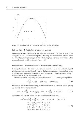
Figure 1.13 Velocity profile for 1-D laminar flow with a moving upper plate.

Solving the 1-D fluid flow problem in MATLAB

simple flow 1D.m solves the 1-D flow example above where the fluid is water ( ρ =
−3
3
3
10 kg/m ,µ = 10 Pa s), the upper plate is stationary, and the separation between plates
is 1 mm. The dynamic pressure gradient is selected to give a Reynolds’ number near 1. The
computed velocity profile is shown in Figure 1.13.

Fill-in (why Gaussian elimination is sometimes impractical)
It is important to note that many sparse systems cannot be placed in a banded form, and
elimination remains costly. For such systems, the iterative techniques discussed later in our
discussion of boundary value problems are preferred. Even if a matrix is banded; however,
elimination may be too costly due to fill-in.
The flow example (1.237) and (1.238) was of the form of a 1-D boundary value problem,
2
d ϕ
− 2 = f (y) ϕ(0) = ϕ 0 ϕ(B) = ϕ B (1.256)
dy
Each row of the linear system resulting from finite differences on a uniform grid of spacing
y has only three nonzero elements
−1 2 −1
A k,k−1 = A k,k = A k,k+1 = b k = f (y k ) (1.257)
( y) 2 ( y) 2 ( y) 2
As is shown in Chapter 6, for the analogous problem on a 2-D domain,
2
2
∂ ϕ ∂ ϕ
2
−∇ ϕ =− − = f (x, y) 0 ≤ x ≤ L 0 ≤ y ≤ H
∂x 2 ∂y 2
BC1 ϕ(0, y) = 0 0 ≤ y ≤ H
BC2 ϕ(L, y) = 0 0 ≤ y ≤ H
(1.258)
BC3 ϕ(x, 0) = 0 0 ≤ x ≤ L
BC4 ϕ(x, H) = 00 ≤ x ≤ L